Both MLE and MAP are answering the same question: given observed data $D$, what’s the “best” single value for some parameter $\theta$ ? They differ in what “best” means.

Maximum Likelihood Estimation (MLE) asks: which $\theta$ makes the observed data most probable?

We treat $\theta$ as a fixed unknown and only look at the likelihood - how well each candidate $\theta$ explains the data we actually saw. There’s no opinion about $\theta$ before seeing data; every parameter value starts on equal footing.

Maximum A Posteriori (MAP) asks: given the data and my prior beliefs, which $\theta$ is most probable?

So MAP is literally MLE with an extra multiplicative factor - the prior $p(\theta)$.

Suppose we flip a coin 3 times and get 3 heads. MLE says the probability to get heads $\hat{p}=1$, because that’s the $p$ maximizing the likelihood $p^3$. That’s technically correct given only the data, but it feels absurd. MAP with, say, a Beta(2,2) prior would pull the estimate toward 0.5, giving something like $\hat{p}=4 / 6$. The prior regularizes against extreme conclusions from small samples.

In $\log$-space, MAP becomes $\log p(D \mid \theta)+\log p(\theta)$. If the prior is Gaussian $p(\theta) \propto \exp \left(-\lambda\lVert \theta\rVert^2\right)$, then $\log p(\theta)$ is just $-\lambda\lVert \theta\rVert^2$ which is an L2 penalty. So MAP with a Gaussian prior is MLE + weight decay. A Laplace prior gives L1 / LASSO. Every time we add weight decay in training, we’re implicitly doing MAP.

Another thing worth mentioning is that both MLE and MAP are point estimate. MLE gives the mode of the likelihood $p(D \mid \theta)$, MAP gives the mode of the posterior $p(\theta \mid D)$. To get a full distribution we need Bayesian inference. So MAP is sometimes called “the lazy person’s Bayesian inference”

Two kinds of latents

The global latent parameter $\theta$

In MAP and MLE, we assume that each $x_i\in D$ was drawn from some distribution $p(x \mid \theta)$. This $\theta$ is parameters in the classical sense , e.g. the mean and variance of a Gaussian, the weights of a neural network, the bias of a coin. These are fixed (in the frequentist view) or random (in the Bayesian view), but either way they parameterize the data distribution globally. Every observation $x_i$ is governed by the same $\theta$. MLE and MAP are primarily about estimating these.

But a single fixed $\theta$ (or multiple $\theta$s) would be too rigid to explain diverse data on its own, the number doesn’t really matter, $\theta$ can be millions of weights in a neural network, but what matters is that it is fixed after training. That leads to a more flexible framework using per-example latent variables.

Per-example latent variables $z_i$

Here, every observation $x_i$ has its own hidden variable $z_i$, the global, fixed (after training) $\theta$ governs how to generate $x_i$ from $z_i$.

Remark: where $z$ comes from is flexible, for example we can sample $z_i$ based on $\theta$ in GMM, or just $p(z)=\mathcal{N}(0, I)$ in standard VAE, or determined (not a sample) by $x$ in standard autoencoder.

The generative story becomes first we sample $z_i$

Then we sample $x_i$ based on $z_i$ and $\theta$

Now here’s the key: we have two kinds of unknowns, and MLE/MAP refer specifically to how we handle $\theta$, not $z$.

Methodology

MLE for $\theta$ says: find the $\theta$ that maximizes the probability of the observed data, after marginalizing out the latents $z$ :

That integral $\int p_\theta(x \mid z) p(z) d z$ is the marginal likelihood of a single observation. We’re summing over all possible latent codes $z$ that could have produced $x_i$, weighted by the prior. So the objective is purely a function of $\theta$.

MAP for $\theta$ just put a prior $p(\theta)$ on the model parameters:

This is just MLE plus a penalty from $p(\theta)$.

The $\theta$ is the target of MLE or MAP not latent $z$. For simple cases (like GMM) where the posterior is tractable, EM algorithm infer both $z$ and $\theta$ from $D$: the E-step handles the per-example latents $z_i$, the M-step handles the global parameters $\theta$. For complex decoders (like neural networks) where the integral $\int p_\theta(x \mid z) p(z) d z$ is intractable, we introduce $q_\phi(z \mid x)$ to approximate the posterior $p_\theta(z \mid x)$ and derive a tractable lower bound on $\log p_\theta(x)$

The right hand side is called ELBO. Detailed calculations can be found From Likelihood to ELBO.

Two kinds of KL

The ELBO uses $D_{\mathrm{KL}}(q \parallel p)$ specifically, but the choice of KL direction has consequences worth examining.

This is an often overlooked issue. We know that KL is not symmetric, means $D_{\mathrm{KL}}(q \parallel p)\neq D_{\mathrm{KL}}(p \parallel q)$. We want $q$ to be “close” to $p$, but the two directions of KL give us fundamentally different meanings of “close.”

$D_{\mathrm{KL}}(q \parallel p)$ - mode-seeking

We’re taking the expectation under $q$ :

This blows up whenever $q(z)>0$ but $p(z) \approx 0$. So $q$ is severely penalized for putting mass where $p$ has none. The solution $q$ avoids any region where $p$ is small, and instead concentrates on a single mode of $p$ where it’s safe. If $p$ is bimodal, $q$ will pick one mode and ignore the other entirely rather than risk straddling the gap between them where $p$ is near zero.

$D_{\mathrm{KL}}(p \parallel q)$ - mass-covering

Now the expectation is under $p$ :

This blows up whenever $p(z)>0$ but $q(z) \approx 0$. So $q$ is penalized for missing any region where $p$ has mass. The solution $q$ spreads out to cover all modes of $p$. If $p$ is bimodal, $q$ will stretch itself wide enough to cover both modes, even if that means putting mass in the gap between them where $p$ is actually low.

The ELBO optimizes the mode-seeking direction $D_{\mathrm{KL}}\left(q_\phi(z \mid x) \parallel p_\theta(z \mid x)\right)$, which means the encoder will lock onto one mode of the true posterior if it’s multimodal.

Classical group-equivariant neural networks enforce pointwise constraints $F(g \cdot x) = \rho(g) \cdot F(x)$, requiring that inputs related by a group element $g$ produce outputs related by the same symmetry. This formulation treats data as isolated points connected by group actions.

In our thesis, we introduce Path Equivariant Networks (PENs), which replace pointwise constraints with pathwise constraints: as data traverses continuous paths on a manifold, network outputs must transform coherently via transport maps. The central theoretical result, presented below, shows that classical group equivariance is recovered from path equivariance under a natural condition on path endpoints: establishing that classical equivariant networks are a special case of the PEN framework.

We present here the complete chain of definitions and proofs leading to this recovery theorem. All notation is defined within this document.

Outline of the Argument

The logical chain proceeds as follows:

1. Define path equivariance (PE). Given a path system $\mathcal{P}$ on input space $X$ and a Lie group $A$ acting on output space $Z$, a map $F: X \to Z$ is PE if traversing any path $\gamma \in \mathcal{P}$ in $X$ induces a continuous transport $a_\gamma: [0,1] \to A$ satisfying $F(\gamma(t)) = a_\gamma(t) \cdot F(\gamma(0))$. (Definition 2.5)

2. Introduce the endpoint condition. If two paths in $G$ share the same endpoints, their transports agree at $t=1$. This allows us to define a map $\rho: G^0 \to A$ by $\rho(g) := a_\gamma(1)$, independent of path choice. (Definitions 3.1–3.2)

3. Prove $\rho$ is a group homomorphism. The path $e \to g_1 g_2$ decomposes as $e \xrightarrow{\gamma_2} g_2 \xrightarrow{\gamma_1 \cdot g_2} g_1 g_2$, and the transport along this concatenation factors as $\rho(g_1) \cdot \rho(g_2)$. (Proposition 4.1)

4. Recover classical equivariance. For any $g \in G^0$ and $x \in X$, choose a path $\gamma$ from $e$ to $g$, evaluate PE at $t = 1$, and apply the endpoint condition to get $F(g \cdot x) = \rho(g) \cdot F(x)$. (Theorem 4.2)

The key insight: classical equivariance relates isolated pairs of points $(x, g \cdot x)$. Path equivariance relates continuous families of points along paths. The endpoint condition collapses path-dependent transport to a point-dependent map $\rho$, recovering the classical setting. Geometrically, the endpoint condition is equivalent to trivial holonomy (a flat connection), and relaxing it yields strictly more general equivariance notions.

1. Preliminaries

Definition 1.1 (Lie Group). A Lie group $G$ is a smooth manifold that is also a group, with smooth multiplication $m: G \times G \to G$ and inversion $i: G \to G$.

Definition 1.2 (Identity Component). The identity component $G^0$ of a Lie group $G$ is the connected component containing the identity element $e$. Since $G$ is a Lie group (hence a topological manifold), $G^0$ is path-connected: for any $g \in G^0$, there exists a continuous path $\gamma: [0,1] \to G$ with $\gamma(0) = e$ and $\gamma(1) = g$.

Definition 1.3 (Group Action). An action of a Lie group $G$ on a space $X$ is a continuous map $\rho: G \times X \to X$ satisfying $e \cdot x = x$ and $(g_1 g_2) \cdot x = g_1 \cdot (g_2 \cdot x)$ for all $g_1, g_2 \in G$, $x \in X$. We write $G \curvearrowright X$.

2. Path Systems and Path Equivariance

Definition 2.1 (Path Reparametrization and Concatenation). If $\gamma: [0,1] \to X$ is a path and $\phi: [0,1] \to [0,1]$ is continuous with $\phi(0) = 0$, $\phi(1) = 1$, the reparametrized path is $\gamma \circ \phi$.

If $\gamma_1, \gamma_2$ are paths with $\gamma_1(1) = \gamma_2(0)$, their concatenation is:

Definition 2.2 (Path System). A path system on a topological space $X$ is a non-empty family of continuous paths $\gamma: [0,1] \to X$ that is closed under reparametrization and concatenation.

Definition 2.3 (Group Path System). Let $G \curvearrowright X$. The group path system is:

Proposition 2.4. The group path system $\mathcal{P}$ is a path system.

Proof. We verify closure under reparametrization and concatenation.

Reparametrization. Let $\gamma_X(t) = \gamma_G(t) \cdot x \in \mathcal{P}$ and let $\phi: [0,1] \to [0,1]$ be continuous with $\phi(0) = 0$, $\phi(1) = 1$. Define $\tilde{\gamma}_G(t) := \gamma_G(\phi(t))$. Then $\tilde{\gamma}_G$ is continuous, $\tilde{\gamma}_G(0) = \gamma_G(\phi(0)) = \gamma_G(0) = e$, and

Concatenation. Let $\gamma_{X,1}(t) = \gamma_{G,1}(t) \cdot x_1$ and $\gamma_{X,2}(t) = \gamma_{G,2}(t) \cdot x_2$ be in $\mathcal{P}$ with $\gamma_{X,1}(1) = \gamma_{X,2}(0)$. The matching condition gives $\gamma_{G,1}(1) \cdot x_1 = e \cdot x_2 = x_2$, so $x_2 = \gamma_{G,1}(1) \cdot x_1$. The concatenation is:

Define the concatenated group path:

We verify: $\tilde{\gamma}G(0) = \gamma{G,1}(0) = e$; and continuity at $t = 1/2$ holds because

Therefore $(\gamma_{X,1} \parallel \gamma_{X,2})(t) = \tilde{\gamma}_G(t) \cdot x_1 \in \mathcal{P}$. $\square$

Definition 2.5 (Path Equivariance). Let $G \curvearrowright X$, let $A$ be a Lie group acting on a manifold $Z$, and let $\mathcal{P}$ be a path system on $X$. A continuous map $F: X \to Z$ is path equivariant with respect to $\mathcal{P}$ if for every $\gamma \in \mathcal{P}$, there exists a continuous transport $a_\gamma: [0,1] \to A$ with $a_\gamma(0) = e_A$ such that

We further assume the transport is base-point independent: for a group path $\gamma_G: [0,1] \to G$, the transport $a_{\gamma_G}$ depends only on $\gamma_G$, not on the choice of $x \in X$.

3. The Endpoint Condition and the Endpoint Map

Definition 3.1 (Endpoint Condition). A path-equivariant map $F$ satisfies the endpoint condition if, for all group paths $\gamma_1, \gamma_2: [0,1] \to G^0$ with $\gamma_1(0) = \gamma_2(0) = e$ and $\gamma_1(1) = \gamma_2(1) = g$, the induced transports agree at $t = 1$:

Definition 3.2 (Endpoint Map). Under the endpoint condition, define $\rho: G^0 \to A$ by

where $\gamma$ is any continuous path in $G^0$ from $e$ to $g$. Since $G^0$ is path-connected, such a path exists for every $g \in G^0$, and the endpoint condition guarantees that $\rho$ is independent of the choice of path.

4. Main Results

Proposition 4.1. The endpoint map $\rho: G^0 \to A$ is a group homomorphism.

Proof. We verify three properties.

(i) Identity. Take the constant path $\gamma(t) = e$ for all $t$. Then $F(\gamma(t) \cdot x) = F(e \cdot x) = F(x)$ for all $t$, so the transport $a_\gamma(t) = e_A$ for all $t$ satisfies the path equivariance condition. Therefore $\rho(e) = a_\gamma(1) = e_A$.

(ii) Multiplicativity. Let $g_1, g_2 \in G^0$. Choose paths $\gamma_1: [0,1] \to G^0$ from $e$ to $g_1$ and $\gamma_2: [0,1] \to G^0$ from $e$ to $g_2$, with corresponding transports $a_{\gamma_1}$ and $a_{\gamma_2}$.

We construct a path from $e$ to $g_1 g_2$ in two stages. First traverse $\gamma_2$ (going $e \to g_2$), then apply the “shifted” path $g_2 \mapsto g_1 g_2$ corresponding to $\gamma_1$. Formally, define:

This is continuous (at $t = 1/2$: $\gamma_1(0) \cdot g_2 = e \cdot g_2 = g_2 = \gamma_2(1)$), starts at $\tilde{\gamma}(0) = e$, and ends at $\tilde{\gamma}(1) = g_1 \cdot g_2$.

Now consider the induced paths in $X$. For any $x \in X$, the path $\tilde{\gamma}(t) \cdot x$ consists of two segments:

• First segment ($t \in [0, 1/2]$): the path $\gamma_2(2t) \cdot x$ starting at $x$. By path equivariance: $F(\gamma_2(2t) \cdot x) = a_{\gamma_2}(2t) \cdot F(x)$. At $t = 1/2$, this gives $F(g_2 \cdot x) = a_{\gamma_2}(1) \cdot F(x) = \rho(g_2) \cdot F(x)$.

• Second segment ($t \in [1/2, 1]$): the path $\gamma_1(2t-1) \cdot (g_2 \cdot x)$ starting at $g_2 \cdot x$. By path equivariance with base-point independence: $F(\gamma_1(2t-1) \cdot (g_2 \cdot x)) = a_{\gamma_1}(2t-1) \cdot F(g_2 \cdot x)$. At $t = 1$, this gives $F(g_1 g_2 \cdot x) = a_{\gamma_1}(1) \cdot F(g_2 \cdot x) = \rho(g_1) \cdot F(g_2 \cdot x)$.

Combining both segments:

On the other hand, by definition of the endpoint map applied to the path $\tilde{\gamma}$ from $e$ to $g_1 g_2$:

Since this holds for all $x \in X$ and all $F(x) \in Z$, we conclude $\rho(g_1 g_2) = \rho(g_1) \cdot \rho(g_2)$.

(iii) Inverses. Let $g \in G^0$ and let $\gamma: [0,1] \to G^0$ be a path from $e$ to $g$. Define the reversed group path $\bar{\gamma}(t) := \gamma(1-t) \cdot \gamma(1)^{-1}$, which satisfies $\bar{\gamma}(0) = \gamma(1) \cdot \gamma(1)^{-1} = e$ and $\bar{\gamma}(1) = \gamma(0) \cdot g^{-1} = g^{-1}$.

Consider the concatenation $\gamma \parallel \bar{\gamma}$, which is a path from $e$ to $e$ (a closed loop). The endpoint condition applied to the constant path $c(t) = e$ and the loop $\gamma \parallel \bar{\gamma}$ gives:

By the composition of transports along the concatenation:

Therefore $\rho(g^{-1}) \cdot \rho(g) = e_A$, which gives $\rho(g^{-1}) = \rho(g)^{-1}$.

This completes the proof that $\rho$ is a group homomorphism. $\square$

Theorem 4.2 (Recovery of Classical Group Equivariance). Let $G \curvearrowright X$ and $A \curvearrowright Z$. Let $F: X \to Z$ be path equivariant with respect to the group path system $\mathcal{P}$ with base-point independent transport, and assume the endpoint condition holds. Then:

where $\rho: G^0 \to A$ is the endpoint map, which is a continuous group homomorphism by Proposition 4.1. This is the classical group equivariance law on $G^0$.

Proof. Fix $g \in G^0$ and $x \in X$. Since $G^0$ is path-connected, there exists a continuous path $\gamma: [0,1] \to G^0$ with $\gamma(0) = e$ and $\gamma(1) = g$.

Consider the group path in $X$:

This satisfies $\gamma_X(0) = e \cdot x = x$ and $\gamma_X(1) = g \cdot x$, and belongs to the group path system $\mathcal{P}$.

Since $F$ is path equivariant, there exists a continuous transport $a_\gamma: [0,1] \to A$ with $a_\gamma(0) = e_A$ such that:

Evaluating at $t = 1$:

By the endpoint condition and the definition of $\rho$ (Definition 3.2):

Therefore:

Since $g \in G^0$ and $x \in X$ were arbitrary, this establishes the classical equivariance law on the identity component $G^0$. $\square$

5. Discussion

The recovery theorem establishes a precise hierarchy of equivariance conditions:

• Path equivariance (Definition 2.5) is the most general: the transport $a_\gamma$ may depend on the entire path $\gamma$, not just its endpoints.
• Classical group equivariance $F(g \cdot x) = \rho(g) \cdot F(x)$ is recovered when the endpoint condition holds: the transport depends only on the endpoint $g = \gamma(1)$, not on the path taken.

The endpoint condition has a natural geometric interpretation. Given two paths $\gamma_1, \gamma_2$ from $e$ to $g$, the concatenation $\gamma_1 \parallel \gamma_2^{-1}$ is a closed loop at $e$. The endpoint condition requires $a_{\gamma_1}(1) = a_{\gamma_2}(1)$, i.e., the transport around any closed loop is trivial. In the language of differential geometry, this corresponds to trivial holonomy, or equivalently, a flat connection on the associated principal bundle.

This perspective suggests an intermediate notion, homotopy equivariance, where the transport depends only on the homotopy class of the path. Homotopic paths induce the same transport, but non-homotopic paths to the same endpoint may differ. When $G^0$ is simply connected, every two paths with the same endpoints are homotopic, and homotopy equivariance coincides with the endpoint condition. When $G^0$ has non-trivial fundamental group $\pi_1(G^0, e)$, the holonomy around topologically distinct loops may be non-trivial, yielding a strictly intermediate framework.

Source: Chapter 4 of “Exploring the Structure in Deep Networks: Group, Manifold and Category Theory,” M.Sc. Thesis, Aalto University, December 2025.

As argued in Part 2: The Group Structure of Neural Networks, valid gradient descent should cross the orbit, because within an orbit all weights are functionally equivalent, this is the reparametrization symmetry of neural networks. In standard training this is trivial: since the objective is to minimize loss, and the loss is constant along orbits, the gradient is automatically orthogonal to orbit directions. No special machinery is needed.

However, this symmetry structure becomes consequential when measuring generalization. Sharpness-Aware Minimization (SAM) (Foret et al., 2021) characterizes generalization by perturbing parameters within an $\epsilon$-ball and measuring the worst-case loss increase. The intuition is that flat minima where the loss is insensitive to perturbation are associated with better generalization (Hochreiter & Schmidhuber, 1997; Keskar et al., 2017).

The problem is that orbit directions are trivially flat: perturbing along an orbit never increases the loss. When we measure sharpness over an $\epsilon$-ball in parameter space, these orbit directions consume volume in the perturbation ball while contributing nothing to the worst-case loss increase.

This has two consequences. First, sharpness measurements are biased low: the landscape appears flatter than it actually is, because the orbit-flat directions pull down the average curvature. Second, sharpness measurements become incomparable across models with similar functional capacity but different widths. A wider network with a larger symmetry group therefore has more trivially flat directions, making its sharpness artificially lower regardless of the actual functional geometry of the loss landscape. This complicates the use of sharpness as a proxy for generalization in neural architecture comparison (Dinh et al., 2017).

To address this, we define sharpness on the quotient manifold $\mathcal{M}=\Theta / G$, restricting perturbations to directions that change the network function.

Compared with full-space sharpness:

we define quotient sharpness:

Here $\mathcal{H}_\theta$ is the orthogonal complement of the orbit tangent space at $\theta$. By confining the perturbation ball to functionally distinct directions, the resulting sharpness measure captures genuine sensitivity of the network function to parameter changes, without the confound of reparametrization symmetry.

Reference

• Foret, P., Kleiner, A., Mobahi, H., & Neyshabur, B. (2021). Sharpness-Aware Minimization for Efficiently Improving Generalization. ICLR 2021.
• Hochreiter, S. & Schmidhuber, J. (1997). Flat Minima. Neural Computation, 9(1), 1–42.
• Keskar, N. S., Mudigere, D., Nocedal, J., Smelyanskiy, M., & Tang, P. T. P. (2017). On Large-Batch Training for Deep Learning: Generalization Gap and Sharp Minima. ICLR 2017.
• Dinh, L., Pascanu, R., Bengio, S., & Bengio, Y. (2017). Sharp Minima Can Generalize for Deep Nets. ICML 2017.

Prologue: What defines a person?

This article originated from a conversation I had with a friend: How should we treat human rights? In philosophy, Kant argued that rational human beings should be treated as an end in themselves, not as a means to something else: a person has inherent dignity. Marx saw it differently: a human being is a socially constructed, creative species-being (Gattungswesen) whose nature is defined by productive labor and social relations. The self is constituted by its surroundings, by its embedding in a social world.

Even though it is controversial, if we let our analogy run wild, there are mathematically two ways of understanding the same object: intrinsic and extrinsic. At least in mathematics, neither is more correct than the other; they are just different representations of the same reality.

What follows is a tour of this idea. I start from a confusion I had when I was a child.

Sailing around the world

In 1522, the remnants of Magellan’s expedition completed the first circumnavigation of the globe. They had demonstrated that the Earth is not “flat” (technically closed in at least one direction) — you can go all the way around.

But this doesn’t prove the Earth is a sphere! How do we know we’re not living on a donut? The easiest (maybe not) way to determine this is to take a picture from space. But obviously people had already determined the shape of the Earth before that. If not by circumnavigation, then how?

Unfortunately, the answer to this question is not as easy as it looks, and we are not prepared to discuss it here.

But it’s definitely doable, even though we don’t introduce how yet. Taking a picture from space and traveling on the surface of the Earth are equivalent ways to know our Earth, corresponding to extrinsic and intrinsic. They both have the full ability to describe an object (not necessarily geometric).

Intrinsic and Extrinsic

Extrinsic lives with ambient space. “Ambient” just means “surrounding.” An ambient space is just a larger space that an object fits in. For example we put a sphere in a 3D Euclidean space so we can parameterize it. The extrinsic view needs ambient space, contingent on the choice of ambient space.

But one fact we must accept: an object exists by itself, ambient space is not necessary for the existence of an object. A sphere is always a sphere whether we put it in 3D Euclidean space, or a distorted high-dimensional space, or no space at all. This is the view of intrinsic.

Roughly, intrinsic properties are determined by the object itself. Extrinsic describes the relationship between the object and its ambient.

Two pictures of gravity

In this section we briefly introduce Einstein’s general relativity and Newton’s perspective (not Newton’s law) to explain gravity. The distinction between intrinsic and extrinsic is not just a mathematical curiosity. It sits at the center of one of the great transitions in physics: from Newton’s picture of gravity to Einstein’s.

In Newton’s picture, space and time are a fixed, flat stage, an absolute backdrop against which physics unfolds. Space is Euclidean, time flows uniformly, and neither is affected by what happens within them. A planet moves through this stage, and gravity is a force that reaches across it and pulls objects off their natural straight-line paths. This is, at its heart, an extrinsic viewpoint: everything is observed against a fixed ambient background, and gravity is a deviation from flatness.

Einstein replaced this entirely with an intrinsic picture. In general relativity, there is no fixed stage. Space and time are not a passive backdrop but a dynamic, curved entity, spacetime, shaped by the distribution of mass and energy through the Einstein field equations. A planet does not sit in spacetime the way a ball sits in a box. The planet and the spacetime around it form one geometric structure.

In this picture, gravity is not a force. Objects in free fall, including light, follow geodesics: the straightest possible paths through curved spacetime. Light curving near a star is not being “pulled” off a straight line. It is traveling as straight as it possibly can. The apparent bending is an artifact of projecting a curved geometry onto flat expectations. There is a famous quote by John Archibald Wheeler “Matter tells spacetime how to curve, spacetime tells matter how to move.”

Two pictures of kernel

In machine learning, given two points $x, y$, a kernel $k(x, y)$ measures how correlated the function values $f(x)$ and $f(y)$ are. If $k(x, y)$ is large, knowing $f(x)$ tells us a lot about $f(y)$. If $k(x, y)$ is near zero, $f(x)$ and $f(y)$ are roughly independent.

In the Gaussian Process context, a kernel must be a covariance function, which is equivalent to saying a kernel must be symmetric positive semi-definite (PSD). Choosing a kernel is choosing what kind of distribution we assume before seeing data. For example, the squared exponential (SE) kernel assumes that nearby points are highly correlated and the correlation decays smoothly like a Gaussian bell curve. A widely-used SE kernel formula is

where $\sigma^2$ controls how much $f$ varies overall, and $\ell$ controls how quickly the correlation decays with distance. They are hyperparameters.

But what does $\lVert x-y\rVert^2$ mean? It is the squared Euclidean distance.

So when we write this formula, we implicitly use the flat Euclidean metric as the measure of similarity.

But recall what a kernel means: it measures how correlated $f(x)$ and $f(y)$ are. It says nothing about distance or space. Naturally, we can try to use kernels on other spaces, for example on a Riemannian manifold, by replacing the Euclidean distance with the geodesic distance:

This immediately leads to a problem: the resulting function is not necessarily PSD, which means it is not a valid kernel (Feragen et al., 2015). The PSD-ness of the Euclidean SE kernel relies on a special algebraic property of Euclidean distance. In other words, the Euclidean SE kernel is an extrinsic formula that breaks when we try to make it intrinsic by naively swapping in the manifold’s own distance.

There is an alternative definition. The Euclidean SE kernel can also be characterized as

where $f$ is the Gaussian process satisfying the SPDE

Here $\Delta$ is the Laplacian, $\mathcal{W}$ is Gaussian white noise, and $\exp \left(-\frac{\kappa^2}{4} \Delta\right)$ is the (rescaled) heat semigroup. The length-scale parameter $\kappa$ controls how far correlations spread.

Every ingredient in this equation is intrinsic. The Laplace-Beltrami operator $\Delta$ is constructed from the metric tensor alone. White noise $\mathcal{W}$ requires only a measure on the space (the Riemannian volume form). No ambient space is needed. This means the equation can be written on any Riemannian manifold by simply by replacing $\Delta$ with the LaplaceBeltrami operator of that manifold, and the resulting kernel is guaranteed to be PSD (Borovitskiy et al., 2020).

Intuitively, the extrinsic view asks “how far apart are these two points?” while the intrinsic view asks “what does smoothing look like on this space?”. On $\mathbb{R}^n$, the intrinsic and extrinsic definitions give exactly the same kernel, but on curved spaces, only the intrinsic one survives.

Reference

• Feragen, A., Lauze, F., and Hauberg, S. (2015). Geodesic exponential kernels: When curvature and linearity conflict. Conference on Computer Vision and Pattern Recognition (CVPR).
• Borovitskiy, V., Terenin, A., Mostowsky, P., and Deisenroth, M. P. (2020). Matérn Gaussian processes on Riemannian manifolds. Advances in Neural Information Processing Systems (NeurIPS).

Part 5 of 5, following Part 1: Prior Knowledge, Part 2: The Group Structure of Neural Networks, Part 3: Path Equivariance, Part 4: A Category Theory Perspective

In this section we connect classical group equivariance, path equivariance (PE), holonomy, and the Single Tangent Space Fallacy [1]. We show that the holonomy group controls the expressivity of PE: when holonomy is trivial, PE reduces to classical group equivariance, the holonomy group captures exactly the information that group equivariance misses in curved spaces. We then use this framework to explain the Single Tangent Space Fallacy – why the single tangent space approach works on Lie groups but fails on general Riemannian manifolds. The group structure of a Lie group naturally ensures trivial holonomy, making path choice irrelevant; on a general Riemannian manifold, parallel transport is path-dependent, and collapsing to a single tangent space discards this information.

Classical Equivariant Neural Networks

Given a group $G$ acting on the data space $x \mapsto g \cdot x$ and simultaneously feature space $v \mapsto \rho(g) \cdot v$ , the classical equivariant neural networks enforce a global symmetry constraint, every layer $F$ satisfies

where $\rho : G \to GL(V)$ is a representation.

This works when the data space is homogeneous - $G$ acts transitively on this space. But many real data spaces are not homogeneous. A robot’s configuration space has regions of free motion and regions near joint limits. A molecular energy landscape has flat basins and sharp saddle points. Forcing the same symmetry everywhere is geometrically wrong: it respects symmetries that don’t exist in flat regions and fails to capture the path-dependence that curvature introduces.

The deeper issue is that features at different points live in different fibers (usually we use tangent space in manifold learning). A feature at $x \in M$ belongs to a fiber $E_x$, and a feature at $y$ belongs to $E_y$. There is no canonical way to compare them, we need a rule for moving vectors between fibers.

That is the reason we introduce path (or parallel transport) equivariance.

Path Equivariance (PE)

PE operates on an associated vector bundle $E = P \times_\rho V$ over a data manifold $M$, where $P \to M$ is a principal $G$-bundle and $\rho : G \to GL(V)$ is a representation. A feature at point $x$ is a vector $v \in E_x \cong V$.

A connection $\nabla$ on $P$ defines parallel transport along paths: given a path $\gamma : [0,1] \to M$, transport is a linear map

that slides vectors from one fiber to another. Crucially (which we will discuss later), $\tau_\gamma$ depends on the entire path $\gamma$, not just its endpoints $\gamma(0)$ and $\gamma(1)$, unless the connection is flat.

A PE layer $F$ acts pointwise: at each $x \in M$, there is a linear map $F_x : E_x \to E_x$. The defining constraint is

for every path $\gamma$ from $x$ to $y$.

In category theory language, we can draw the square commutes:

The parallel transport defines a functor $\tau : \mathcal{P}(M) \to \mathbf{Vect}$ , the layer $F$ which is a linear map $F_x : E_x \to E_x$ is a natural transformation from the functor $\tau$ to itself. The PEN constraint IS naturality.

Note: the $\pi^{-1}$ arrows connecting the data level to the feature level aren’t really a “map” in the usual sense — $\pi : E \to M$ is the bundle projection, and $\pi^{-1}(x) = E_x$ is the fiber. The fiber assignment is itself part of what the functor $\tau$ does.

The constraint is local and path-dependent. It does not require a global group action. It does not assume the data space is homogeneous. It asks only that the network respects the geometry encoded in the connection.

Holonomy Controls Expressivity

Now we need to ask a fundamental question about PEN: is transport path-dependent?

The PEN constraint applies to all paths, but not all paths are equally informative. For an open path $\gamma : x \to y$, the constraint $F_y \circ \tau_\gamma = \tau_\gamma \circ F_x$ couples two different maps at two different points. It tells us how $F_x$ and $F_y$ relate, but says nothing about what $F_x$ must commute with on its own.

Closed loops are different. When $\gamma$ starts and ends at $x$, the transport $\tau_\gamma : E_x \to E_x$ is an endomorphism of a single fiber, and the constraint collapses to $F_x \circ \tau_\gamma = \tau_\gamma \circ F_x$ - a commutation condition on $F_x$ alone. The holonomy group $\mathrm{Hol}x(\nabla)$ collects all such $\tau\gamma$ over every closed loop at $x$, so the PEN constraint on loops becomes

This has the same algebraic form as global equivariance, but with $\mathrm{Hol}_x(\nabla)$ in place of $G$. Since $\mathrm{Hol}_x(\nabla) \subseteq G$, the constraint is generically weaker - the network has more freedom.

But why do loops at a single point tell us anything about transport between two different points? Because any two paths between the same endpoints compose into a loop. Take $\gamma_1, \gamma_2$ from $x$ to $y$ and form $\gamma = \gamma_1 \cdot \gamma_2^{-1}$. Its transport is

so $\tau_{\gamma_1} = \tau_{\gamma_2}$ if and only if $\tau_\gamma = \mathrm{id}$. Path-dependence between two points is detected by holonomy at one point.

Back to our question: is transport path-dependent? If every loop at $x$ gives trivial transport, then $\mathrm{Hol}_x(\nabla) = \lbrace e\rbrace$, transport is path-independent everywhere, and global equivariance suffices (PEN reduces to global equivariance). If some loop rotates a vector, different paths give different transports, and PEN is genuinely necessary.

The size of the holonomy group varies across the manifold, controlled by curvature. In flat regions where $\mathrm{Hol}_x$ is small, $F_x$ must commute with few elements and has high expressivity. In curved regions where $\mathrm{Hol}_x$ is large, $F_x$ must commute with many elements and is tightly constrained. PEN performs a spatially adaptive trade-off between expressive freedom and geometric fidelity, mediated by curvature through holonomy.

Reduction to Global Group Equivariance

(Path-Independent Condition) Given two paths $\gamma_1, \gamma_2$ from $x$ to $y$, we say the transport satisfies path-independent condition if

The destination vector depends only on where we start and where we end, not on how we get there.

On simply connected $M$, path-independence is equivalent to three other conditions, all describing the same phenomenon from different angles:

1. $\mathrm{Hol}(\nabla) = \lbrace e\rbrace$. Every closed loop transports vectors back to themselves. (trivial holonomy)
2. The connection is flat (zero curvature)
3. PEN collapses to classical equivariance: paths carry no more information than their endpoints

The Single Tangent Space Fallacy

This section draws on the paper Unraveling the Single Tangent Space Fallacy [1].

A common workaround for data on curved manifolds: pick a base point $p$, map everything to $T_pM$ via the logarithmic map $\mathrm{Log}_p$, and work in that single flat vector space. Geometrically, this imposes a flat connection on the tangent bundle - transport from any point to $p$ is the $\mathrm{Log}$ map, independent of path. The holonomy group is trivial: $\mathrm{Hol} = \lbrace e\rbrace$, the path-independent condition holds trivially, and PEN reduces to global equivariance. The cost is distortion. Points far from $p$ are mapped with increasing error, and the curvature information, which encodes genuine structure in the data, is discarded.

The tangent bundle approach keeps each point’s tangent space $T_xM$ separate. A vector at $x$ and a vector at $y$ live in different spaces, and comparing them requires parallel transport via the connection along a specific path. On a curved manifold this transport is path-dependent, holonomy is non-trivial, and PEN is the architecturally principled framework for respecting this structure.

The paper Unraveling the Single Tangent Space Fallacy makes the case concretely in robotics learning: the single-tangent-space approach is acceptable when the manifold is a Lie group, but introduces severe distortion on general Riemannian manifolds.

Lie Groups Case: It Is Fine

A Lie group $G$ acts on itself by left multiplication $L_g : h \mapsto gh$. Its differential $dL_g : T_eG \xrightarrow{\sim} T_gG$ canonically identifies every tangent space with the Lie algebra $\mathfrak{g} = T_eG$. There is no choice, no ambiguity, no path-dependence - the map is determined by $g$ alone. The connection is flat. The path-independent condition holds automatically: a path from $e$ to $g$ is fully characterized by $g$, and $f(g \cdot x) = \rho(g) \cdot f(x)$ works because $g$ encodes everything.

This is why the single tangent space approach is harmless on Lie groups — we’re not killing any holonomy, because there was none to begin with. The group structure of Lie group gives a unique identification between fibers (tangent space). The multiplication $e \mapsto g$ gives us $dL_g$ with no ambiguity, the parallel transport along any path from $e$ to $g$ agrees with $dL_g$.

Riemannian Manifolds Case: Why Fallacy

A general Riemannian manifold does not have group structure. There is no self-action and no canonical map between $T_xM$ and $T_yM$. We must specify a path $\gamma$ and use the Levi-Civita connection to transport. Different paths give different results. No single group element $g$ summarizes the relationship between $x$ and $y$, the path carries independent information. The classical equation $f(g \cdot x) = \rho(g) \cdot f(x)$ breaks down, and PEN becomes necessary.

Path-Independent Condition, Flat Mapping, and Group Representation

The path-independent condition says all paths with the same endpoints produce the same transport. When it holds, transport from $x$ to $y$ depends only on the pair $(x, y)$, not on the path. Pick a base point $x_0$: the transport $T(x_0, y) : E_{x_0} \to E_y$ is now well-defined for each $y$, and these transports compose consistently - $T(x_0, z) = T(y, z) \circ T(x_0, y)$ - so they form a group action on the fibers.

On a Lie group $G$, this is exactly what happens. The pair $(x, y)$ is captured by a single group element $xg = y$, the transport is a differential (pushforward) $dL_g$, and the path is redundant. The connection is flat, so the path-independent condition holds automatically and group equivariance is valid.

On a general curved Riemannian manifold, the transport $T(x, y)$ is not well-defined - it depends on the route. No single group element summarizes the relationship between $x$ and $y$, and standard group equivariance breaks down.

On simply connected $M$, the following conditions are equivalent:

1. The connection is flat.
2. $\mathrm{Hol}(\nabla) = \lbrace e\rbrace$. Every closed loop transports vectors back to themselves.
3. PEN collapses to classical equivariance: paths carry no more information than their endpoints.
4. Transport is path-independent: $\tau_{\gamma_1} = \tau_{\gamma_2}$ for all paths sharing the same endpoints.
5. Transport defines a consistent group action on fibers: $T(x, y) : E_x \to E_y$ depends only on $(x, y)$, and these maps compose as a group.

When any of these fails, the connection is curved, transport is path-dependent, no consistent group action exists, and PEN is necessary.

One important distinction: flatness here is a property of the connection on the bundle, not of the base space. The manifold itself can be curved, e.g.$SO(3)$ is not flat as a Riemannian manifold, yet can still carry a flat connection on its tangent bundle . The geometry of the base space and the geometry of the connection are independent.

Summary

In classical equivariance, a path from $e$ to $g$ is summarized by the group element $g$ - the path is redundant, and the equivariance condition $f(g \cdot x) = \rho(g) \cdot f(x)$ mentions only $g$. In PEN, the path $\gamma$ itself is the fundamental object. The equivariance condition

is indexed by paths, not group elements. The parallel transport $\tau_\gamma$ plays the role that $g$ played in classical equivariance, but depends on the entire path, not just its endpoints. This is a genuine generalization: when the connection is flat, $\tau_\gamma$ depends only on endpoints, paths collapse to group elements, and PEN recovers classical equivariance. When the connection is curved, $\tau_\gamma$ carries strictly more information, and the path is irreplaceable.

The holonomy group $\mathrm{Hol}(\nabla)$ measures the gap between these regimes. Trivial holonomy means group equivariance suffices. Non-trivial holonomy means it doesn’t - and PEN provides a spatially adaptive inductive bias, constrained where curvature demands it, expressive where geometry permits it.

Spherical Cow in a Vacuum

The theoretical framework is clean. The practical question is harder: where does the connection come from? With group equivariance, the workflow is straightforward : domain knowledge gives us the symmetry group, and we build layers that respect it. With PEN, the connection is not typically known in advance.

• Connection known. The data lives on a manifold with a known Riemannian metric e.g. robot arms, molecular dynamics, general relativity. The Levi-Civita connection is determined, parallel transport can be computed analytically, and PEN layers commute with it exactly. This might be the cleanest case.

• Connection constrained. The manifold $M$ is known (e.g., SPD matrices, a Lie group quotient), but there is a family of possible connections. Domain knowledge constrains the holonomy group to a subgroup of $G$. PEN provides the architectural scaffold; the specific connection is selected or learned within the constrained family.

• Connection learned. The data manifold itself is unknown. The manifold, the bundle, and the connection are learned jointly. This is the most ambitious regime. PEN provides an inductive bias: whatever connection the network learns, the layers automatically respect its parallel transport.

What PEN buys over group equivariance

Group equivariance imposes the same symmetry constraint everywhere, it assumes the data space is homogeneous. Many real spaces are not. A robot arm near a joint limit is highly curved and constrained; far from joint limits, it is nearly flat and free. A globally equivariant network cannot adapt to this variation. PEN can, because the holonomy constraint automatically tightens where curvature is high and loosens where it is low. The result is a spatially adaptive inductive bias instead of a uniform one.

Reference

[1] Jaquier, N., Rozo, L., & Asfour, T. (2024). Unraveling the Single Tangent Space Fallacy: An Analysis and Clarification for Applying Riemannian Geometry in Robot Learning. arXiv preprint arXiv:2310.07902. https://arxiv.org/abs/2310.07902

We first review the geometry of linear maps via SVD, then recall PSD matrices, and finally apply both to the Euclidean distance problem.

A real matrix

encodes a linear map

The map can collapse dimensions. The rank $r=\operatorname{rank}(M)$ is the number of linearly independent columns (or rows).

• Column space (image) $\mathcal{C}(M)=\lbrace M x \mid x \in \mathbb{R}^n\rbrace \subseteq \mathbb{R}^d$ is an $r$-dimensional subspace.
• Null space (kernel) $\mathcal{N}(M)=\lbrace x \in \mathbb{R}^n \mid M x=0\rbrace$ has dimension $(n-r)$.

So although inputs live in $n$ dimensions, only an $r$-dimensional slice survives after the transformation.

If we perform SVD on $M$:

SVD decomposes any linear map into three steps: rotate, stretch, rotate. Specifically:

$V^T$ (or equivalently, $V$ ) is an orthogonal matrix $\left(V^T V=I\right)$ with shape $n\times n$, it represents

• pure rotation ($\det=1$, $SO$ group),
• or an improper rotation, i.e., rotation composed with reflection ($\det=-1$)

$V^Tx$: rotate $x$

$\Sigma$ is a descending singular values diagonal matrix ( $\sigma_1 \geq \sigma_2 \geq \ldots$ ). It has same rank $r$, means stretch along the principal axes.

• Components aligned with the singular directions are stretched or compressed by $\sigma_i$.
• Components orthogonal to these directions are completely eliminated (mapped to zero).

$\Sigma V^Tx$: stretch $V^Tx$ along $r$ dimensions, and possibly reduce dimensions(project from $\mathbb{R}^n$ to $\mathbb{R}^d$)

$U$: another orthogonal matrix, but in $\mathbb{R}^d$

An eigenvector of a matrix $A$ is a special vector that remains in the same direction (or is reversed) when transformed by $A$:

Geometrically, eigenvectors are the directions that survive a linear transformation unchanged (up to scaling); the eigenvalue $\lambda$ tells you the scaling factor. A zero eigenvalue $\lambda$ and its eigenvector $v$ means the matrix maps direction $v$ to zero.

Positive Semidefinite (PSD) Matrices ($S_{+}^n$)

The following statements are equivalent:

• The matrix $A \in S^n$ is positive semidefinite $(A \succeq 0)$.
• For all $x \in \mathbb{R}^n, x^T A x \geq 0$.
• All eigenvalues of $A$ are nonnegative.
• All $2^{n-1}$ principal minors of $A$ are nonnegative.
• There exists a factorization $A=B^T B$.

Remark: The second condition ($x^TAx \geq 0$ for all $x$) is generally impractical to check directly; the eigenvalue or factorization conditions are used in practice.

Euclidean distance problem

Consider $n$ points, each in dimension $d$:

Can a set of points be identified uniquely from all the pairwise distances between them? Yes, and these points are equivalent up to rigid transformations

Gram matrix

For a data matrix $X\in \mathbb{R}^{d \times n}$,

Thus $\operatorname{rank}(\tilde{G})=\operatorname{rank}\left(X^T X\right)=\operatorname{rank}(X)=d$

Remark: The entries of the Gram matrix are inner products: $\tilde{G}_{ij} = \langle x_i, x_j \rangle$. This makes the PSD property immediate – Gram matrices are always PSD by construction ($x^T \tilde{G} x = x^T X^T X x = \lVert Xx\rVert^2 \geq 0$).

In practice, we often observe pairwise distances rather than coordinates. Given $D^{(2)} \in \mathbb{R}^{n \times n}$ as the pointwise squared distance matrix, $D^{(2)}$ is symmetric (i.e., $D^{(2)} \in S^n$), but not necessarily PSD.

Geometric centering matrix

where $I_n$ is the $n \times n$ identity matrix and $\mathbb{1}$ is the vector of ones.

Remark: $\operatorname{rank}(J)=n-1$. Multiplying by $J$ centers the data (subtracts the mean).

According to classical multidimensional scaling (cMDS), the Gram matrix can be recovered from squared distances via double centering (see e.g., Borg & Groenen, Modern Multidimensional Scaling, Ch. 12):

The key idea: expanding $D^{(2)}{ij} = \lVert x_i - x_j\rVert^2 = \lVert x_i\rVert^2 - 2\langle x_i, x_j \rangle + \lVert x_j\rVert^2$ and applying the centering matrix $J$ eliminates the squared-norm terms, leaving only the inner products $\tilde{G}{ij} = \langle x_i, x_j \rangle$.

Recall gram matrix is defined as $\tilde{G}:=X^TX\in\mathbb{R}^{n\times n}$, so our goal is to find a $\hat{X}$ has structure $\tilde{G}=\hat{X}^T \hat{X}$. In this case, $\hat{X}$ is a rigid transformation of the original points

Compute the eigendecomposition

Because $\tilde{G}$ is PSD, its eigenvalues are nonnegative.

Recall Gram matrix $\tilde{G}$ has rank $d$ , so we have $\lambda_1$ to $\lambda_d$

Define the $n \times d$ matrix of the first $d$ eigenvectors $Q_d$ and the square root diagonal matrix:

We can write the Gram matrix as

So

Each row of $\hat{X}$ gives the coordinates of a point in $\mathbb{R}^d$, recovered from distances alone. The reconstruction is unique up to rigid transformations (rotations and reflections), which is the best we can hope for – distances are invariant under such transformations.

This technique underlies applications in molecular distance geometry (reconstructing protein structures from NMR data), sensor network localization, and dimensionality reduction via MDS.

Notation

Define sample space as the set of all possible outcomes, denoted as $\Omega$. Define the measure $(\Omega, \mathcal{F}, P)$ A sample is a single element $\omega \in \Omega$ An event is a subset $A \subseteq \Omega$ (more precisely, $A \in \mathcal{F}$) A random variable $X: \Omega \rightarrow \mathbb{R}^d$ is a measurable function. A value $x \in \mathbb{R}^d$ is a specific point in the target space. With $x$, an event is a measurable set, denoted

which is the pre-image $X^{-1}({x})$ A probability measure is a triple $(\Omega, \mathcal{F}, P)$ where $P: \mathcal{F} \rightarrow[0,1]$ A probability of event is $P(X=x)\in [0,1]$ A distribution of $X$, denoted as $P_X$, is a pushforward measure induced by a random variable: When we have a random variable $X: \Omega \rightarrow \mathbb{R}^d$, it induces a probability measure on $\mathbb{R}^d$ :

for measurable sets $A \subseteq \mathbb{R}^d$.

We have a problem: an event can happen even if its probability is 0.

For example, in continuous $X$:

So we can’t assign positive probability to individual points. To solve this, we introduce the Probability Density Function (PDF) The PDF $p_X(x)$ is a function such that:

for any measurable set $A$.

Note:

• $p_X(x)$ is not a probability. It’s a density, so it can be greater than 1
• $p_X(x) d x$ represents the probability of being in an infinitesimal region around $x$. Formally

Their relation:

In this essay, we denote a latent variable as $X$, observation data as $Y$.

$p(\cdot)$

This is one of the most abused notations in probability and machine learning. Strictly speaking, the lowercase $p$ denotes PDF, the capital $P$ denotes probability, the lowercase $x$ denotes a value of random variable, the capital $X$ means random variable.

For Bayes’ theorem (more rigorous explanation check Probability-1): In statistics, usually we write $p(X, Y)=p(Y \mid X) p(X)$, means “the relationship between these density functions” In ML, usually we write $p(x, y)=p(y \mid x) p(x)$, is shorthand for

where:

• $p_{X, Y}: \mathbb{R}^{d_1} \times \mathbb{R}^{d_2} \rightarrow[0, \infty)$ is joint density function
• $p_{Y \mid X}: \mathbb{R}^{d_2} \times \mathbb{R}^{d_1} \rightarrow[0, \infty)$ is conditional density function
• $p_X: \mathbb{R}^{d_1} \rightarrow[0, \infty)$ is marginal density function
• $x, y$ are specific values these random variables can take.

If condition is an observed $x$, we usually write $p(x, Y)=p(Y \mid x) p(x)$

But in ML, lowercase $p$ and $x$ are used for everything: $p(x)$ can mean density function, or distribution, or probability masses $p(X=x)$. $p(X)$ can denote distribution, or density function. The meaning depends on context.

I can understand what $Y$ means, it’s our observation, the data we collected, but what do you mean by “ latent variable? Is it what we observe or what we believe?

Here is the abstract part of probability theory: we don’t care (and usually don’t know) what $X$ really is, we can think of it as an object that satisfies certain properties, for example:

• $X\sim \mathcal{N}(0,I)$
• $x\in X$, $P(x)=0.1$

The Learning Story: take VAE for example

What’s our observation (What do we know)?

We observe dataset $Y=\lbrace y_1, y_2, \ldots, y_n\rbrace$

What’s our assumption?

We assume the distribution of the latent variable $X$, for example, $p(X)=\mathcal{N}(0, I)$, called prior. Also we assume $Y \mid X$ follows some distribution, for example $p(Y \mid X=x)= \mathcal{N}\left(f(x), \sigma^2 I\right)$, called likelihood.

Why we need to specify $X=x$ ?

Because our assumption is a causal/generative structure where $Y$ depends on $X$. The distribution of $Y$ changes based on what value $X$ takes.

What do we want to know?

We want to learn the parameters of function $f$ in $\mathcal{N}\left(f(x), \sigma^2 I\right)$.

Examples of $f$:

Linear model: $f(x)=W x+b$

• Learn: weight matrix $W$ and bias $b$
• This is Probabilistic PCA or Factor Analysis

Neural network: $f(x)=\mathrm{NN}_\theta(x)$

• Learn: neural network weights $\theta$
• This is a Variational Autoencoder (VAE)

Gaussian Process: $f \sim \mathcal{G} \mathcal{P}(m, k)$

• Learn: kernel parameters
• This is Gaussian Process Latent Variable Model (GPLVM)

Set up

Our question: What’s the distribution of $Y$? Or, what’s the probability of observing $y\in Y$, i.e., $p(y)$?

The idea: $Y$ is generated by a latent variable $X$. Let’s write $p(y)$ using $X$. In a more concrete (or abstract?) saying: let’s detect $Y$ using $X$ in a probabilistic way.

Prior (assumed, fixed):

Likelihood (form assumed, parameters learned):

where $f_\theta$ is a neural network with weights $\theta$ Observe:

Unknown (to be learned):

REMARK: Technically all $p(\cdot)$ and $q(\cdot)$ in formulas are density not probability, but densities satisfy the same algebraic rules as probabilities (Bayes, marginalization, chain rule), so we say they are probability, but calculate them as density. Why density? We will see it later…

By Bayes’ theorem, the joint distribution:

where:

• $p(x)=\mathcal{N}(0, I)$ is our prior
• $p_\theta(y \mid x)=\mathcal{N}\left(f_\theta(x), \sigma^2 I\right)$ is our likelihood, parameterized by $\theta$

The marginal (called marginal likelihood, or evidence) is a integral:

Back to the question: What’s the probability of observing $y$ under parameter $\theta$? The answer is: We follow the trace $x$ generates $y$. But we need to consider all possible latent $x$ that could have generated $y$.

Objective: Maximum Likelihood Estimation (MLE) of the parameters $\theta$. Let’s formalize this objective.

Define the Likelihood Function:

A bit confusing: $\mathcal{L}(\theta ; y)=p_\theta(y)$ has different interpretations:

• As a function of $y$ with $\theta$ fixed : It’s a probability distribution
• As a function of $\theta$ with $y$ fixed : It’s a likelihood function In learning story $y$ is known, we want to learn $\theta$, so it is a likelihood function. Likelihood is NOT a probability distribution over $\theta$, its integral generally is not 1, it’s just a positive function of $\theta$.

Maybe more confusing, we have different types of likelihood:

1. Conditional likelihood: $p_\theta(y \mid x)$ : probability of $y$ given $x$ and $\theta$
2. Marginal likelihood: $p_\theta(y)=\int p_\theta(y \mid x) p(x) d x$: probability of $y$ given $\theta$ (marginalizing $x$ )
3. Likelihood function: $\mathcal{L}(\theta ; y)=p_\theta(y)$ : same as (2), but viewed as a function of $\theta$

Recall our Objective: Maximum Likelihood Estimation (MLE), find $\theta$ that maximizes the likelihood of the observed data.

Which likelihood?

First we compare MLE and MAP

MLE (Maximum Likelihood Estimation) - Frequentists’ perspective Objective: Find $\theta$ that maximizes likelihood

Philosophy:

• $\theta$ is a fixed (unknown, we need to learn to step by step) value
• No probability distribution over $\theta$
• Find single “best” estimate

MAP (Maximum A Posteriori) - Bayesians’ perspective Objective: Find $\theta$ that maximizes posterior

Philosophy:

• $\theta$ is a random variable with distribution
• Prior beliefs about $\theta$ encoded in $p(\theta)$
• Update beliefs using data

DIGRESSION: The distinction between frequentist and Bayesian perspectives are also reflected in the symbols. There are two ways to denote conditional probability: $p_\theta(y)$ and $p(y \mid \theta)$, numerically they’re the same, but differ in philosophy. $p_\theta(y)$ : Frequentist view:

• $\theta$ is a fixed but unknown parameter (not random)
• The subscript indicates “the density function indexed/parameterized by $\theta$”
• $\theta$ lives in parameter space, not in probability space

• We cannot write $p(\theta)$ because $\theta$ is not a random variable $p(y \mid \theta)$ : Bayesian view:

• $\theta$ is a random variable with its own distribution
• This is a conditional density: density of $y$ given $\theta$
• We can write $p(\theta)$ (prior), $p(\theta \mid y)$ (posterior), etc.
• Bayes’ theorem applies:

Modern machine learning commonly use hybrid approach, which is also called Type II Maximum Likelihood: Maximize $p_\theta(y)=\int p_\theta(y \mid x) p(x) d x$ over $\theta$

Bayes’ Equation: Inferring Latents Given Data

where

• Posterior: $p_\theta(x \mid y)$ - what we want (latent given data)
• Likelihood: $p_\theta(y \mid x)$ - conditional likelihood
• Prior: $p(x)$ - prior on latents
• Evidence: $p_\theta(y)$ - marginal likelihood

The likelihood Function: $\mathcal{L}(\theta ; y)=p_\theta(y)$, with different perspectives of $y$ and $\theta$ , is

• Probability of data y given parameters $\theta$
• Notation: $p(y \mid \theta)$ or $p_\theta(y)$
• A function of $\theta$ (with $y$ fixed)
• NOT a probability distribution over $\theta$

So, the “likelihood” in Maximum Likelihood Estimation, is NOT the (conditional) likelihood is Bayes’s equation related to $x$ and $y$, instead, it is the evidence, aka marginal likelihood. Maximum Likelihood Estimation actually maximize the likelihood function $\mathcal{L}(\theta ; y)$ , which is $p_\theta(y)$ viewed as a function of $\theta$.

Collect all the observations $y_i$, our objective is:

Or in log form:

But in general, this integral is intractable.

Why?

$p_\theta\left(y_i \mid x\right)$ contains a neural network; basically, we can believe that everything that contains a neural network is not analytically integrable. Also, we can’t use the sampling method (Monte Carlo), if we want to sample from the prior $p(x)$ to approximate

where $x^{(l)} \sim p(x)=\mathcal{N}(0, I)$. We want $p_\theta\left(y \mid x^{(l)}\right)$ to be as high as possible, so it’s an effective sample. But the latent space (all possible $x$ ) is very broad. The set of $x$ that generate a specific $y$ (for example, an image )is very narrow. Most random samples from $p(x)$ give tiny $p_\theta\left(y \mid x^{(l)}\right)$, making the sampling method exponentially inefficient.

One guiding principle from engineering: we don’t need to be the best, we just need to be good enough.

Evidence Lower Bound (ELBO)

We make another assumption: $q_\phi(x \mid y)$ as a known distribution. For example $q_\phi(x \mid y)=\mathcal{N}\left(\mu_\phi(y), \operatorname{diag}\left(\sigma_\phi^2(y)\right)\right)$ , its only parameter is $\phi$.

The variational trick: Using $q_\phi(x \mid y)$ to approximate the true posterior $p_\theta(x \mid y)$ .

Multiply and divide by $q_\phi(x \mid y)$ inside the integral:

where $\mathbb{E}{q\phi(x \mid y)}\left[\log p_\theta(y \mid x)\right]-D_{K L}\left(q_\phi(x \mid y) \lVert p(x)\right)$ is called ELBO.

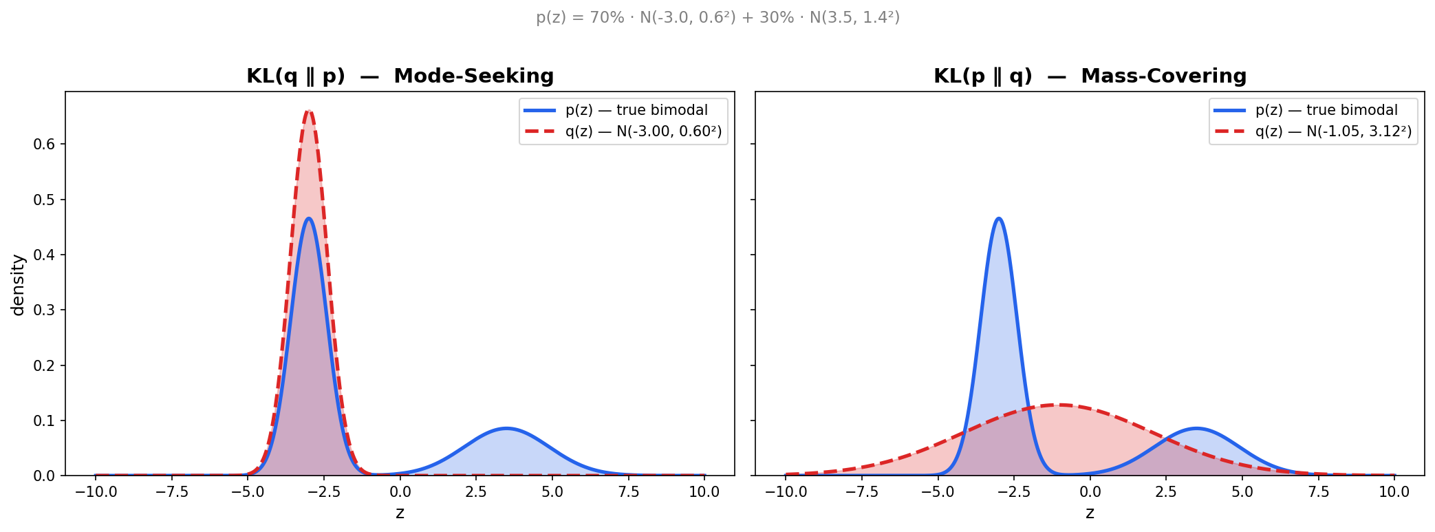
Note: Here we define KL divergence $D_{KL}$, which measures the difference between two probability distributions (but not a distance). There are many ways to measure differences between probabilities, KL divergence is a good one: analogously, it is the “Euclidean distance” in probability space.

REMARK: There is another sloppy notation. Technically $p(\cdot)$ and $q(\cdot)$ are density function, not probability. When we write

what we actually mean is

where $Q_\phi$ is the probability measure, the $q_\phi(x \mid y)$ is its density, such that $Q_\phi(d x)=q_\phi(x \mid y) d x$ Most time we can interchangeably use probability and density. But in some cases, for example in this expectation trick, $p(\cdot)$ must be density. Another non-trivial case is reparameterization: If $Y=h(X)$ for some transformation $h$ , then

• Probability is preserved: $P(Y \in h(A))=P(X \in A)$
• Density transforms with a Jacobian:

Densities are not invariant under reparameterization.

Now we know $\log p_\theta(y)\geq \mathrm{ELBO}$, so ELBO is a lower bound on $\log p_\theta(y)$,

Next we recover $\log p_\theta(y)$ from ELBO

Substitute using Bayes’ equation:

Since $\log p_\theta(y)$ doesn’t depend on $x$, it’s constant with respect to the expectation over $q_\phi(x \mid y)$ :

This gives us the key equation:

where ELBO is a scalar-valued function of parameters $\theta$ and $\phi$.

Since $D_{K L} \geq 0$, the same conclusion as before: ELBO is always a lower bound on $\log p_\theta(y)$. When $q_\phi(x \mid y)=p_\theta(x \mid y)$, i.e., our approximate posterior exactly matches the true posterior, ELBO equals the true log-likelihood.

We observe an interesting phenomena in this equation. Since the left side is fixed when we vary $\phi$ :

Therefore:

When we increase ELBO by changing $\phi$ , we decreases KL divergence simultaneously!

But all components of this equation depend on $\theta$. When we increase ELBO by changing $\theta$, $\log p_\theta(y)$ increases, but at the same time, the true posterior $p_\theta(x \mid y)$ is moving, so KL might increase or decrease. But overall, we’re making the model better!

Now, our objective becomes

Methodology

Recall the ELBO formula:

This looks more complex, we need to optimize with respect to both $\theta$ and $\phi$. Is it tractable?

Yes! We untangle it item by item.

KL item

The KL part is relatively easy. For example if we take both Gaussian:

• $q_\phi(x \mid y)=\mathcal{N}\left(\mu_\phi(y), \operatorname{diag}(\sigma_\phi^2(y))\right)$
• $p(x)=\mathcal{N}(0, I)$ The KL divergence (for diagonal covariance Gaussian vs standard normal) is:

where $\mu=\mu_\phi(y)$ and $\sigma^2=\sigma_\phi^2(y)$. Note: this closed form assumes $q_\phi$ has diagonal covariance; the general case with a full covariance matrix is more complex. This is differentiable with respect to $\phi!$ We can compute gradients directly.

Expectation item

The expectation item needs to be more careful. By definition

A little break…

Let’s clarify notations before we go further.

What is $q_\phi(x \mid y) ?$

It’s our assumption used to surrogate the true posterior $p_\theta(x \mid y)$ where

• $\phi$ is the parameter that defines the function
• $y$ is the observation, aka the conditional variable, which is given/fixed when we write this expression
• $x$ is the argument of the function. This is what the density function takes as input and produces density values for, $x$ ranges over all possible latent codes We can think of it as a function:

Given fixed $\phi$ (parameters) and fixed $y$ (observation), this is a function of $x$ :

• Input: a latent code $x$
• Output: density value $q_\phi(x \mid y)$

What is $\log p_\theta(y \mid x)$?

Similarly we can think it as a Function:

Given fixed $\theta$ and fixed $x$, this is a function of $y$ :

• Input: an observation $y$
• Output: density value $p_\theta(y \mid x)$

What is $\int q_\phi(x \mid y)\log p_\theta(y \mid x)dx$ ?

It is the average value of $\log p_\theta(y \mid x)$ when $x$ is distributed according to $q_\phi(x \mid y)$ . We’re not picking a specific $x$ . We’re computing a weighted average over all possible $x$ values, where the weights are given by $q_\phi(x \mid y)$.

Expectation item again

By definition

Parameter $\theta$ is relatively easy: $\nabla_\theta \mathbb{E}{q\phi(x \mid y)}\left[\log p_\theta(y \mid x)\right]$. We focus on $\phi$.

First we try to find what is the best $\phi$ for this item , or equally , update $\phi$ via the trajectory

Recall $p_\theta(y \mid x)=\mathcal{N}\left(f_\theta(x), \sigma^2 I\right)$ , since $f_\theta(x)$ doesn’t depend on $\phi$,

A common choice $q_\phi(x \mid y)=\mathcal{N}\left(\mu_\phi(y), \sigma_\phi^2(y)\right)$, but this is still hard because $\mu$ and $\sigma$ are neural networks (encoder). The main issue is that we are integrating target variable.

How can we avoid integration?

We hope the integration can be written as expectation, then expectation can be approximated by Monte Carlo.

Reparameterization trick

This is a really smart and elegant idea.

What can we usually do with a distribution? We sample a point from it. But this “sample” operation is really confusing—how do we do it? Ideally, the sampled element should preserve all information about its distribution, so we know this point is truly sampled from the correct distribution, not randomly generated. Another issue is that, in machine learning, we need to update the parameters of the distribution using this sampled point. How can we achieve that?

The problem: $\phi$ appears in the distribution we’re sampling from ($q_\phi$), so we can’t differentiate through the sampling.

The solution: reparameterize so that $\phi$ appears only in a deterministic transformation of a fixed noise distribution.

In mathematics, we constantly use different perspectives to view identical objects. For example, $q_\phi(x \mid y)$ is both a function of $x$ with codomain $[0,\infty)$, and also a distribution $\mathcal{N}\left(\mu_\phi(y), \sigma_\phi^2(y)\right)$ with parameter $\phi$. The value of the function $q_\phi$ gives $x$, is identical to, the probability of sampling $x$ from the distribution $q_\phi$.

Based on this idea, instead of sampling:

We use a deterministic function:

where $\epsilon \sim p(\epsilon)=\mathcal{N}(0, I)$ is a fixed noise variable that doesn’t depend on $\phi$. This is valid because they give the same distribution for $X$. Instead of sampling $x$, we now sample $\epsilon$.

The original expectation:

Can be rewritten as:

We changed variables in the integral!

Key difference: Now $\phi$ appears only in the integrand $g(\phi, \epsilon, y)$, NOT in the distribution $p(\epsilon)$ . Since $p(\epsilon)$ doesn’t depend on $\phi$ , we can rewrite gradient of expectation as the expectation of gradient

Now we can use Monte Carlo Estimation. By sampling $\epsilon$ from $p(\epsilon)$, which is $\mathcal{N}(0,I)$:

where $\epsilon^{(1)}, \ldots, \epsilon^{(L)} \sim \mathcal{N}(0, I)$

Why Monte Carlo works now?

Recall our building

Sample $\epsilon\sim p(\epsilon)$ to estimate $\left[\log p_\theta(y \mid g(\phi, \epsilon, y))\right]$ is the same as sample $x \sim q_\phi(x \mid y)$ to estimate $\left[\log p_\theta(y \mid x)\right]$. Initially, $q_\phi\left(x \mid y\right)$ might output random mean, samples from $q_\phi$ don’t reconstruct well, causing high loss. But during the training, $q_\phi\left(x \mid y\right)$ concentrates around $x$ values where $p_\theta\left(y \mid x\right)$ is large, reaching our final goal $q_\phi(x \mid y) \approx p_\theta(x \mid y)$. This is actually related to importance sampling.

For simplicity, we set $L=1$.

where $\epsilon \sim \mathcal{N}(0, I)$ is sampled once per gradient computation.

Now our update trajectory in expectation item is

We can build $\mu_\phi$ and $\sigma_\phi$ as neural networks, take this item as loss function, sample $\epsilon \sim \mathcal{N}(0, I)$, given a fixed $\theta$, this equation is solvable.

But wait, $\theta$ also a unknown variable.

True, we need to optimize both $\theta$ and $\phi$ simultaneously, recall our objective:

We can make joint gradient descent . In each gradient step:

• Update $\phi: \phi^{(t+1)}=\phi^{(t)}+\alpha_\phi \cdot \nabla_\phi$ ELBO
• Update $\theta: \theta^{(t+1)}=\theta^{(t)}+\alpha_\theta \cdot \nabla_\theta$ ELBO

Thus we can learn $\phi$ and $\theta$ simultaneously.

Note: In this case two parameters cooperate (both improve the same goal), it looks like EM algorithm but actually not. An adversarial case is GAN where two parameters against each other.

1. Bayesian Network

Bayesian Network(BN) is composed of Directed Acyclic Graph (DAG) and Conditional Probability Tables (CPT)

In the DAG, nodes represent events, and edges represent dependencies between nodes. Each event happens (or does not happen) with conditional probability $\mathbb{P}$, where the conditional probability is given by CPT.

Why conditional probability in CPT?

Because in a Bayesian Network, events happen sequentially. The sequence of nodes implies the sequence of events. When building the BN, an event can be observed only after observing its parents (happening or not), which means every event probability (except the sources) in the CPT is a conditional probability. The CPT encodes prior conditional probabilities based on the DAG structure. After the BN is built, we can condition on observed evidence to update these probabilities.

One can think of CPT as prior knowledge; its probabilities may change as we acquire more observations. We write $P(AB)$ for the joint probability $P(A \cap B)$ throughout this article.

Example A simple BN with DAG:

A --> B

and CPT:

We can not get ${P}(B)$ directly from CPTs, but we can calculate it using Bayes’ Rule and Law of total probability

2. Independent or conditional independent?

For example, originally we have $P(A)=0.5, P(B)=0.5$. Then something happened, $P(B)=0.9$. Because $A$ and $B$ are independent, $P(A)$ is not affected by the change of $P(B)$, still $P(A)=0.5$.

Case 1

Given a BN with DAG:

A --> B

and CPT:

Are events $A$ and $B$ independent or not? Or, is $P(B)$ affected by the change of $P(A)$?

For $P(B)$, by Bayes’ Rule and Law of total probability:

Similar argument for $P(A)$ as independence is symmetric.

So $A$ and $B$ are not independent.

Case 2

Given a BN with DAG:

A --> B --> C

and CPT:

Are $A$ and $C$ independent or not? Or, is $P(C)$ affected by the change of $P(A)$?

For $P(C)$, by Bayes’ Rule and Law of total probability:

But we don’t know $P(B)$ yet. So using Bayes’ Rule and Law of total probability again:

The change of $P(A)$ leads to the change of $P(B)$ (because $A\ B$ are not independent), and thus leads to the change of $P(C)$ (because $B\ C$ are not independent).

So $A$ and $C$ are not independent.

Are $A$ and $C$ independent or not given $B$? Or, is $P(C)$ affected by the change of $P(A)$ given $P(B)$?

We can think “Given $B$” as we refresh the probability of $B$, which is different from the prior $P(B)$ calculated by CPT. Formally, we condition on $B$, replacing the prior $P(B)$ with the observed value. (Loosely speaking, $P(B)$ is “fixed” after given) Now we can calculate $P(C)$ directly using

So $A$ and $C$ independent given $B$. Formally we say $A$ and $C$ are conditionally independent given $B$

Case 3

Given a BN with DAG:

A <-- B --> C

and CPT:

Are $A$ and $C$ independent or not? Or, is $P(C)$ affected by the change of $P(A)$?

For $P(A)$, by Bayes’ Rule and Law of total probability:

For $P(C)$, by Bayes’ Rule and Law of total probability:

Observing $A$ updates our belief about $B$ (since $B$ is $A$’s parent, Bayes’ rule lets us infer $B$ from $A$), which in turn updates our belief about $C$. So the change of $P(A)$ does affect $P(C)$

So $A$ and $C$ are not independent.

Are A and C independent or not given B? Or, is P(C) affected by the change of P(A) given P(B)?

Now we know the (“fixed”)value of $P(B)$. We can calculate $P(A)$ (or $P(C)$) using $P(B)$ without hesitation. Intuitively, the impact of $A$ on $C$ was “blocked” by a known $B$.

So, $A$ and $C$ are conditionally independent given $B$

Case 4

Given a BN with DAG:

A --> B <-- C

and CPT:

Are A and $C$ independent or not? Or, is $P(C)$ affected by the change of $P(A)$?

Intuitively, $A$ and $C$ are source nodes, meaning they are not directly affected by any other nodes; their occurrences have no conditions. Also, we can directly find $P(A)$ and $P(C)$ from the CPT. The change of probability of one does not affect the other.

How about I use the argument in the previous example: ‘$A$ and $B$ are not independent, $B$ and $C$ are not independent, so the change of $A$ affects $C$ ‘?

$P(B)$ is determined by CPT and the joint probability distribution of $AC$, we can not calculate $P(B)$ simply by CPT and $P(A)$. Even if $P(A)$ changes, we don’t know how it will affect $P(B)$, therefore, we don’t know how it will affect $P(C)$.

So $A$ and $C$ are independent.

Are $A$ and $C$ independent or not given $B$? Or, is $P(C)$ affected by the change of $P(A)$ given $P(B)$?

Now we know the value of $P(B)$ and it is “fixed”. $P(B)$ depends on $A$ and $C$. If we change $P(A)$, $P(C)$ would also be changed because conditioning on $B = b$ induces a constraint: $P(A, C \mid B = b) \propto P(B = b \mid A, C) P(A) P(C)$, which couples $A$ and $C$ even though they were marginally independent.

This is the “explaining away” effect: if two independent causes both contribute to an observed effect, learning about one cause changes our belief about the other. For example, if a disease can be caused by either gene A or virus C, and we observe the disease (B), then learning the patient has gene A makes virus C less likely.

So $A$ and $C$ are not independent given $B$.

The node $B$ in structure $A\rightarrow B\leftarrow C$ is called a collider.

3. Summary

These case-by-case rules are formalized as d-separation (directional separation), the standard framework for reading off conditional independencies from a DAG.

$A\rightarrow B$ , $A$ and $B$ are not independent.

$A\rightarrow B \rightarrow C$, $A$ and $C$ are not independent. $A$ and $C$ are conditionally independent given $B$

$A\leftarrow B\rightarrow C$, $A$ and $C$ are not independent. $A$ and $C$ are conditionally independent given $B$

$A\rightarrow B \leftarrow C$, $A$ and $C$ are independent. $A$ and $C$ are not independent given $B$

The general rule: a path between two nodes is blocked (d-separated) if it contains either (1) a non-collider that is conditioned on, or (2) a collider that is not conditioned on (and has no conditioned descendant). Two nodes are conditionally independent given a set of observed nodes if and only if every path between them is blocked.

Definition: A set $S \subseteq \mathbb{R}^n$ is convex if for every pair of points $x_1$ and $x_2$ in $S$, the entire line segment between them also lies in $S$. Formally,

The intersection of convex sets is convex.

Given a convex set $S$, a point $x \in S$ is called an extreme point if the only way it can appear as a convex combination

is if $x_1=x_2=x$. In other words, $x$ cannot be represented as a “nontrivial” mixture of two distinct points in $S$. Intuition: any point in a convex set can be represented as a point on a line segment, the extreme point can only be represented as its own segment

Examples

For any non-zero $a \in \mathbb{R}^n$ and $b \in \mathbb{R}$, the set

• $\lbrace x \in \mathbb{R}^n: a^T x \leq 0\rbrace$ is a linear halfspace
• $\lbrace x \in \mathbb{R}^n: a^T x \leq b\rbrace$ is an affine halfspace. All these sets are convex. If $n \geq 2$, then they have no extreme points.

The nonnegative orthant $\mathbb{R}_{+}^n:=\lbrace x \in \mathbb{R}^n: x_i \geq 0 \text{ for } i=1, \ldots, n\rbrace$ is a convex cone.

The sublevel set $\lbrace x : x^T A x + b^T x + c \leq 0\rbrace$, where $A \succeq 0$, is convex.

A set $S \subseteq \mathbb{R}^n$ is a cone if $\lambda \geq 0, x \in S$ implies $\lambda x \in S$. Not all cones are convex sets

The set $S_{+}^n$ (PSD) matrices is a convex cone.

Linear programming (LP)

Linear programming (LP) is a special kind of convex optimization. It optimizes a linear function over $\mathbb{R}_{+}^n$ (the nonnegative orthant) subject to linear constraints. The set of all points that satisfy the constraints of an optimization problem is called a feasible region. If the feasible region is non-empty, then the LP is called feasible.

Primal LP formulation

where $c \in \mathbb{R}^n, A \in \mathbb{R}^{m \times n}, b \in \mathbb{R}^m$ and $x \in \mathbb{R}^n$ is the variable over which the optimization is performed.

Dual LP formulation

where $c \in \mathbb{R}^n, A \in \mathbb{R}^{m \times n}, b \in \mathbb{R}^m$ and $y \in \mathbb{R}^m$ is the variable over which the optimization is performed. (This can be derived via Lagrange multipliers.)

Weak duality

For any feasible $x$ in the primal and feasible $y$ in the dual, compare their objective:

Intuition: the dual objective gives a lower bound Short proof: $b^T y=y^T b=y^T(A x)=\left(A^T y\right)^T x \leq c^T x$

Strong duality

If both primal and dual problems are feasible, means

• the primal set $\lbrace x \mid A x=b, x \geq 0\rbrace$ is non-empty
• the dual set $\lbrace y \mid A^T y \leq c\rbrace$ is non-empty. Then they achieve exactly the same optimal value. REMARK: Every linear program (that is feasible and bounded) is strong duality

Semidefinite programming (SDP)

SDP generalizes LP by replacing the nonnegative orthant $\mathbb{R}+^n$ with the cone of positive semidefinite matrices $S+^n$.

Semidefinite programming (SDP) is a special kind of convex optimization problem with nice properties. It optimizes a linear function over $S_{+}^n$ subject to linear constraints.

We consider $S^n$ with the trace inner product

Primal SDP formulation

A semidefinite program (SDP) in its standard (primal) form typically looks like:

where $C, A_i \in S^n, b_i \in \mathbb{R}$ and $X \in S^n$ is the variable over which the optimization is performed.

Or equivalently (the first form using the trace inner product is standard in optimization theory; the second using a linear matrix inequality is common in control theory):

where

• $x \in \mathbb{R}^m$ is the variable,
• $c \in \mathbb{R}^m$ is a given cost vector,
• $F_0, F_1, \ldots, F_m$ are symmetric matrices (of the same dimension $n \times n$ ),
• $F(x) \succeq 0$

Example:

Dual SDP formulation

where $C, A_i \in S^n, b_i \in \mathbb{R}$ and $y \in \mathbb{R}^m$ is the variable over which the optimization is performed.

Example:

Weak duality

The primal objective evaluated at any feasible matrix $X$ is greater than the dual objective evaluated at any feasible vector $y$. The primal objective evaluated at any feasible matrix $X$ gives an upper bound for the optimum of $b^T y$ of the dual problem. The dual objective evaluated at any feasible vector $y$ gives a lower bound for the optimum of $\langle C, X\rangle$ of the primal problem.

Strong duality

A primal SDP formulation is called strictly feasible if there exists $X>0$ that satisfies the linear constraints. A dual SDP formulation is called strictly feasible if there exists $y$ such such that $C-\sum_i A_i y_i>0$. If both the primal and dual problems are strictly feasible, then their optimal solutions are equal.

Application

Euclidean distance problem

From Distances to Coordinates (Euclidean) Recall the Euclidean distance matrix completion problem. If $D^{(2)}$ misses some data, we cannot use cMDS to find the points. We can write the entries of a squared distance matrix in terms of Gram matrix:

The existence of a point configuration in dimension $d$ is equivalent that the Gram matrix $G$ is of rank at most $d$.

So the problem becomes

SDP relaxation

The rank condition is not a linear constraint. We need to relax it:

This relaxation allows the points to embed in $\mathbb{R}^k$ for some $k > d$.

One can apply cMDS to the solution obtained by the SDP relaxation to obtain a solution in $\mathbb{R}^d$. However, the previous SDP does not try to find a solution of low rank.

Rank minimization heuristics

Flatten the graph associated with a partial Euclidean distance matrix by pulling the vertices of the graph as far from each other as possible. Formally, we want to maximize

And we can prove that

REMARK: Often minimize rank $(G)$ is replaced by minimize $\operatorname{Tr}(G)$, which is called the nuclear norm heuristic. Geometric interpretation of minimizing $\operatorname{Tr}(G)$ is bringing vertices as close together as possible. Conversely, maximizing $\operatorname{Tr}(G)$ pushes points apart, favoring higher embedding dimension.

So now we obtain the following SDP:

Nearest Euclidean distance matrix problem(EDM)

A quadratic SDP approach to find the nearest EDM is

PCA

Recall Principal Component Analysis Consider an $n \times p$ centered data matrix $X$, where rows of $X$ contain results for different repeats of the experiment and columns of $X$ record different features.

The covariance matrix is

which is a $p\times p$ matrix

Let $\Sigma \in S_{+}^n$ be a covariance matrix. Variance in the direction of a unit vector $u \in \mathbb{R}^n$ is $u^T \Sigma u$.

First principal component is the direction that explains the most variance. The principal components are normalized eigenvectors of data’s covariance matrix or equivalently the right singular vectors of $X$.

PCA in a SDP view:

• Principal components are linear combinations of all variables
• We are trying to maximize the variance by a particular linear combination of the input variables (a direction) while constraining the number of nonzero coefficients in this combination.

Let $\Sigma \in S_{+}^n$ be a covariance matrix. We want to maximise the variance in the direction of the vector $x \in \mathbb{R}^n$. So we have a SDP:

($\operatorname{Card}(x)$ denotes the number of non-zero entries of $x$)

But this optimization problem is hard because of the cardinality constraint. Consider $X=x x^T$ :

• $X \succeq 0$
• $\operatorname{Rank}(X)=1$
• $\lVert x\rVert_2=1 \Leftrightarrow \operatorname{Tr}(X)=1$
• $\operatorname{Card}(x) \leq k \Leftrightarrow \operatorname{Card}(X) \leq k^2$
• $x^T \Sigma x=\operatorname{Tr}(\Sigma X)$

So we have an equivalent formulation:

Now the convex objective $x^T \Sigma x$ becomes linear objective $\operatorname{Tr}(\Sigma X)$ Nonconvex constraint $\lVert x\rVert_2=1$ becomes linear constraint $\operatorname{Tr}(X)=1$ But problem is still nonconvex. We need to relax the rank and cardinality constraints

Semidefinite relaxation

$X=x x^T$ and $\operatorname{Tr}(X)=1 \Rightarrow\lVert X\rVert_F=1$ $x \in \mathbb{R}^n, \operatorname{Card}(x)=k \Rightarrow\lVert x\rVert_1 \leq \sqrt{k}\lVert x\rVert_2$ $\operatorname{Card}(X) \leq k^2 \Rightarrow \mathbf{1}^T|X| \mathbf{1} \leq k\lVert X\rVert_F=k$

Relaxed SDP for PCA:

The optimal value to SDP will be an upper bound on the optimal value of the variational problem. Let $X_1$ be the solution to SDP and $x_1$ the dominant eigenvector. Since we replaced $\operatorname{Card}(X) \leq k^2$ by the relaxed constraint $\mathbf{1}^T|X| \mathbf{1} \leq k$, then we might not have $\operatorname{Card}\left(X_1\right) \leq k^2$ and $\operatorname{Card}\left(x_1\right) \leq k$. If $\operatorname{Card}\left(x_1\right) \geq k$, we can just use “simple thresholding” to set small entries to 0

Iteration (deflation):

• $\Sigma_1=\Sigma$ to find $x_1$
• $\Sigma_2=\Sigma_1-\left(x_1^T \Sigma_1 x_1\right) x_1 x_1^T$ to find $x_2$
• …

This deflation removes the variance explained by $x_1$, so the next SDP finds the direction of maximum remaining variance. We can add orthogonality constraints $x_i^T x_j=0$ for $i \neq j$ to the optimization problem for all the previously found sparse principal components $x_1, \ldots, x_k$.

Part 4 of 4, following Part 1: Prior Knowledge, Part 2: The Group Structure of Neural Networks, Part 3: Path Equivariance

In this section we use category theory to formalize and unify the prior knowledge, group structure, and path equivariance frameworks from the preceding parts. Although highly abstract, the categorical perspective is surprisingly clear: it gives a name to all the structures we have been building. A model is a functor, and a good model is one whose layers are natural transformations. The equivariance conditions we have discussed throughout are instances of naturality – the same commuting square, in different guises. This gives us a high-level language for reasoning about what a model preserves and what it discards.

A parable about maps

Imagine two cartographers, each tasked with mapping the same mountain range. Cartographer A produces a topographic map: contour lines, elevation, slope. Cartographer B produces a road map: highways, intersections, distances between towns. Both maps represent the same territory, but they preserve different structure. The topographic map preserves elevation relationships; the road map preserves connectivity and distance along roads. Neither is “wrong.” Each is faithful to a specific kind of structure in the original terrain.

Now imagine a third person, not a cartographer but a philosopher of cartography, who asks: “What does it mean to make a map? What does any map preserve, regardless of whether it’s topographic or road-based? Is there a language for talking about ‘structure preservation’ itself, without committing to which structure?”

That philosopher is doing (a portion of) category theory.

This final article steps back from the specific mathematics of groups and manifolds to ask a more basic question: what is a model? Not “what is this model” but “what does it mean for any model to be faithful to the structure of its domain?” The answer turns out to unify everything we have discussed (symmetry, equivariance, path equivariance, composition) into a single framework where the central concept is almost embarrassingly simple: a good model is one that preserves structure of observed data, and the mathematical word for “structure-preserving map” is natural transformation.

The question behind the question

Throughout this series, we have seen the same idea in different guises.

In Part 2 (group structure): a network layer $F$ should commute with symmetry actions, $F(g \cdot x) = \rho(g) \cdot F(x)$. The layer should preserve the group structure of the data.

In Part 3 (path equivariance): a network should transport representations coherently along paths, $F(\gamma(t)) = a_\gamma(t) \cdot F(\gamma(0))$. The layer should preserve the geometric structure of the data manifold.

These look like different conditions, but they share a common shape: apply the structural change, then the map should equal apply the map, then the structural change. Commuting squares. The conditions differ only in what kind of structure is being preserved: a group action, a path transport, a topological invariant.

Category theory is the mathematics that captures this commonality. It says: forget the specific kind of structure. Ask only: what are the objects, what are the structure-preserving maps between them, and what does it mean for a map to be “natural,” to commute with all the structural maps at once?

The language: objects, arrows, functors, naturality

Let me give the minimum vocabulary needed, stripped of formalism.

A category is a world of things (objects) and relationships between them (morphisms/arrows). The category of vector spaces has vector spaces as objects and linear maps as arrows. The category of topological spaces has spaces as objects and continuous maps as arrows. The category of smooth manifolds has manifolds as objects and smooth maps as arrows. What makes each category different is not the objects themselves but what counts as a valid arrow, what structure the arrows preserve.

A functor is a map between categories that preserves the arrow structure. It sends objects to objects and arrows to arrows, such that composition and identity are respected. In our context: a dataset with a $G$-symmetry is a functor from the one-object category $\mathbf{B}G$ (whose arrows are the group elements) into the category of topological spaces. The functor sends the single object to the data space $X$ and sends each group element $g$ to the map $g \cdot -$ on $X$. This is a compact way of saying “$X$ is a space with a $G$-action,” but the categorical language bundles the space and the action into a single object (the functor), which turns out to be exactly the right packaging.

A natural transformation is a map between functors that commutes with all the structural arrows. If $F$ and $E$ are two functors from $\mathbf{B}G$ to some category (two $G$-spaces), a natural transformation $\alpha: F \Rightarrow E$ is a map $\alpha: F() \to E()$ such that for every $g$:

Read this out loud: “apply the symmetry then the map” equals “apply the map then the symmetry.” This is the equivariance condition. It was always a naturality condition. We just didn’t have the language to see it.

Equivariance is naturality

This is the central observation, and it deserves to be stated plainly.

When a practitioner builds a G-CNN and imposes $F(g \cdot x) = \rho(g) \cdot F(x)$, they are not inventing a special constraint for neural networks. They are requiring that their network layer be a natural transformation between functors. The commuting square, the diagram that says “act then map equals map then act,” is the same diagram in category theory and in equivariant deep learning. The conditions are identical. The vocabulary is different.

Why does this matter? Because category theory comes with a toolkit that was developed over decades for reasoning about natural transformations, and that toolkit now applies directly to neural networks.

Composition is free. If layer $\alpha: F \Rightarrow E$ is a natural transformation and layer $\beta: E \Rightarrow H$ is a natural transformation, then $\beta \circ \alpha: F \Rightarrow H$ is automatically a natural transformation. In plain language: stacking equivariant layers gives an equivariant network. This is obvious when we say it in ML terms, but the categorical proof is one line; it follows from the universal properties of natural transformations. The correctness of deep equivariant architectures is a consequence of how arrows compose in functor categories.

Invariant pooling is a limit. When a network pools over group orbits (summing or averaging over all rotations of a feature, for instance) it is computing a categorical limit in the functor category. The universal property of limits guarantees that the result is invariant, and that any other invariant map factors through it. This gives a principled justification for why sum-pooling over orbits (as in DeepSets) is the “right” way to achieve invariance: it is the universal one.

What models really are

Let me push the philosophical point further, because I think it reveals something about deep learning that the purely technical perspective misses.

A child learning to recognize cats does not memorize pixel arrays. They extract an abstract concept, “cat-ness,” that generalizes to cats never seen before. What makes this possible is that the child’s internal representation preserves the relevant structure of the visual world while discarding the irrelevant. The cat is the same cat whether seen from the left or the right, in sunlight or shadow, large or small in the visual field. The child’s model is invariant to pose, illumination, and scale, but sensitive to the features that distinguish cats from dogs.

A neural network, at its best, does the same thing. A CNN’s translation equivariance means it doesn’t care where in the image a feature appears; it preserves spatial relationships while discarding absolute position. A group-equivariant network’s symmetry means it doesn’t care which orientation the object is in; it preserves identity while discarding pose.

Category theory gives this the sharpest possible formulation: a model is a functor, and a good model is one whose layers are natural transformations. The functor maps from the structured world of data (with its symmetries, paths, and geometric constraints) to the structured world of representations (with its own symmetries and constraints). Naturality, the commuting square condition, is what ensures the map is faithful to the structure. Not faithful to the raw data (that would be memorization) but faithful to the relationships in the data (that is generalization).

This is why the categorical perspective matters beyond its technical utility. It tells us what we are doing when we design a neural network: we are choosing which structure to preserve and which to discard, and the architecture is the formal expression of that choice. The functor is the map. The natural transformation is the constraint that makes it honest.

Unifying the series

The four articles in this series can now be seen as four views of the same subject.

Part 1 (prior knowledge) asked: what does a neural network assume before training? Every design choice (architecture, activation, regularization) is prior knowledge. Category theory says: prior knowledge is the choice of source and target categories and the structure-preserving conditions imposed on the functor.

Part 2 (group structure) formalized one kind of structure: algebraic symmetry. The symmetry group of a network, and how it reduces from $\mathrm{GL}(n)$ through activation and regularization, describes which algebraic structure the model preserves. Category theory says: this is the choice of the indexing category $\mathbf{B}G$ and the study of the functor category $[\mathbf{B}G, \mathbf{C}]$.

Part 3 (path equivariance) generalized from algebraic to geometric structure: paths on manifolds, fiber bundles, content-pose decomposition. Category theory says: this is the enrichment of the indexing category from a group (discrete arrows) to a path category (continuous arrows), and the naturality condition generalizes equivariance to path-equivariance.

Part 4 (this article) steps back and sees them all as instances of one idea: models are functors, good layers are natural transformations, and the entire design of a neural network is a choice of which structure to preserve.

The fact that group equivariance, path equivariance, and compositional structure all reduce to the same categorical concept (naturality) is not a coincidence. It reflects something deep about what learning is. Learning is not curve fitting. Learning is the discovery of structure-preserving maps from the world to a representation. Category theory is the mathematics of such maps.

Coda: the shape of constraints

Let me close with the idea that started this series.

Prior knowledge is not what the model learns from data. It is what humans teach the model by choosing its structure. A fully general network can learn anything in theory; prior knowledge means it doesn’t have to. By constraining the model to a subspace of function space (the subspace of translation-equivariant functions, or rotation-equivariant functions, or path-smooth functions) we give it a smaller world to search. If our knowledge is correct, the optimal solution lives in that subspace, and the model finds it faster, with less data, and with better generalization. Prior knowledge doesn’t add to the model; it removes everything the model doesn’t need.

Every model is a hypothesis. Every design choice is prior knowledge. Every prior encodes a structural assumption. What category theory adds is the recognition that these structural assumptions have a shape: the shape of the indexing category, the shape of the commuting diagram, the shape of the functor.

When we choose a group $G$ and build a G-CNN, the shape is $\mathbf{B}G$, a single object with $G$’s worth of self-loops. When we choose path equivariance on a manifold, the shape is richer, a category of paths with composition by concatenation. When we compose equivariant layers into a deep network, the composition is functorial: structure preservation propagates through depth.

The shape of constraints is what separates a model that memorizes from a model that understands. Category theory doesn’t tell us which shape is right for a given problem; that is the domain expert’s job, the human knowledge that no amount of data can replace. But it tells us that once we’ve chosen the shape, the rest (the equivariance conditions, the composition rules, the invariance guarantees) follows by naturality.

And naturality is just a commuting square: act then map equals map then act. Everything else is commentary.

This concludes the five-part series based on the thesis “Exploring the Structure in Deep Networks: Group, Manifold and Category Theory” (Aalto University, 2025).