MAP and MLE

Both MLE and MAP are answering the same question: given observed data $D$, what’s the “best” single value for some parameter $\theta$ ? They differ in what “best” means.

Maximum Likelihood Estimation (MLE) asks: which $\theta$ makes the observed data most probable?

\[\hat{\theta}_{\mathrm{MLE}}=\arg \max _\theta p(D \mid \theta)\]

We treat $\theta$ as a fixed unknown and only look at the likelihood - how well each candidate $\theta$ explains the data we actually saw. There’s no opinion about $\theta$ before seeing data; every parameter value starts on equal footing.

Maximum A Posteriori (MAP) asks: given the data and my prior beliefs, which $\theta$ is most probable?

\[\hat{\theta}_{\mathrm{MAP}}=\arg \max _\theta p(\theta \mid D)=\arg \max _\theta p(D \mid \theta) p(\theta)\]

So MAP is literally MLE with an extra multiplicative factor - the prior $p(\theta)$.

Suppose we flip a coin 3 times and get 3 heads. MLE says the probability to get heads $\hat{p}=1$, because that’s the $p$ maximizing the likelihood $p^3$. That’s technically correct given only the data, but it feels absurd. MAP with, say, a Beta(2,2) prior would pull the estimate toward 0.5, giving something like $\hat{p}=4 / 6$. The prior regularizes against extreme conclusions from small samples.

In $\log$-space, MAP becomes $\log p(D \mid \theta)+\log p(\theta)$. If the prior is Gaussian $p(\theta) \propto \exp \left(-\lambda\lVert \theta\rVert^2\right)$, then $\log p(\theta)$ is just $-\lambda\lVert \theta\rVert^2$ which is an L2 penalty. So MAP with a Gaussian prior is MLE + weight decay. A Laplace prior gives L1 / LASSO. Every time we add weight decay in training, we’re implicitly doing MAP.

Another thing worth mentioning is that both MLE and MAP are point estimate. MLE gives the mode of the likelihood $p(D \mid \theta)$, MAP gives the mode of the posterior $p(\theta \mid D)$. To get a full distribution we need Bayesian inference. So MAP is sometimes called “the lazy person’s Bayesian inference”

Two kinds of latents

The global latent parameter $\theta$

In MAP and MLE, we assume that each $x_i\in D$ was drawn from some distribution $p(x \mid \theta)$. This $\theta$ is parameters in the classical sense , e.g. the mean and variance of a Gaussian, the weights of a neural network, the bias of a coin. These are fixed (in the frequentist view) or random (in the Bayesian view), but either way they parameterize the data distribution globally. Every observation $x_i$ is governed by the same $\theta$. MLE and MAP are primarily about estimating these.

But a single fixed $\theta$ (or multiple $\theta$s) would be too rigid to explain diverse data on its own, the number doesn’t really matter, $\theta$ can be millions of weights in a neural network, but what matters is that it is fixed after training. That leads to a more flexible framework using per-example latent variables.

Per-example latent variables $z_i$

Here, every observation $x_i$ has its own hidden variable $z_i$, the global, fixed (after training) $\theta$ governs how to generate $x_i$ from $z_i$.

Remark: where $z$ comes from is flexible, for example we can sample $z_i$ based on $\theta$ in GMM, or just $p(z)=\mathcal{N}(0, I)$ in standard VAE, or determined (not a sample) by $x$ in standard autoencoder.

The generative story becomes first we sample $z_i$

\[z_i \sim p(z)\]

Then we sample $x_i$ based on $z_i$ and $\theta$

\[x_i \sim p_\theta\left(x \mid z_i\right)\]

Now here’s the key: we have two kinds of unknowns, and MLE/MAP refer specifically to how we handle $\theta$, not $z$.

Methodology

MLE for $\theta$ says: find the $\theta$ that maximizes the probability of the observed data, after marginalizing out the latents $z$ :

\[\hat{\theta}_{\mathrm{MLE}}=\arg \max _\theta p(D \mid \theta)=\arg \max _\theta \prod_i \int p_\theta\left(x_i \mid z\right) p(z) d z\]

That integral $\int p_\theta(x \mid z) p(z) d z$ is the marginal likelihood of a single observation. We’re summing over all possible latent codes $z$ that could have produced $x_i$, weighted by the prior. So the objective is purely a function of $\theta$.

MAP for $\theta$ just put a prior $p(\theta)$ on the model parameters:

\[\hat{\theta}_{\mathrm{MAP}}=\arg \max _\theta p(\theta \mid D)=\arg \max _\theta\left[\prod_i \int p_\theta\left(x_i \mid z\right) p(z) d z\right] p(\theta)\]

This is just MLE plus a penalty from $p(\theta)$.

The $\theta$ is the target of MLE or MAP not latent $z$. For simple cases (like GMM) where the posterior is tractable, EM algorithm infer both $z$ and $\theta$ from $D$: the E-step handles the per-example latents $z_i$, the M-step handles the global parameters $\theta$. For complex decoders (like neural networks) where the integral $\int p_\theta(x \mid z) p(z) d z$ is intractable, we introduce $q_\phi(z \mid x)$ to approximate the posterior $p_\theta(z \mid x)$ and derive a tractable lower bound on $\log p_\theta(x)$

\[\log p_\theta(x) \geq \mathbb{E}_{q_\phi(z \mid x)}\left[\log p_\theta(x \mid z)\right]-D_{\mathrm{KL}}\left(q_\phi(z \mid x) \parallel p(z)\right)\]

The right hand side is called ELBO. Detailed calculations can be found From Likelihood to ELBO.

Two kinds of KL

The ELBO uses $D_{\mathrm{KL}}(q \parallel p)$ specifically, but the choice of KL direction has consequences worth examining.

This is an often overlooked issue. We know that KL is not symmetric, means $D_{\mathrm{KL}}(q \parallel p)\neq D_{\mathrm{KL}}(p \parallel q)$. We want $q$ to be “close” to $p$, but the two directions of KL give us fundamentally different meanings of “close.”

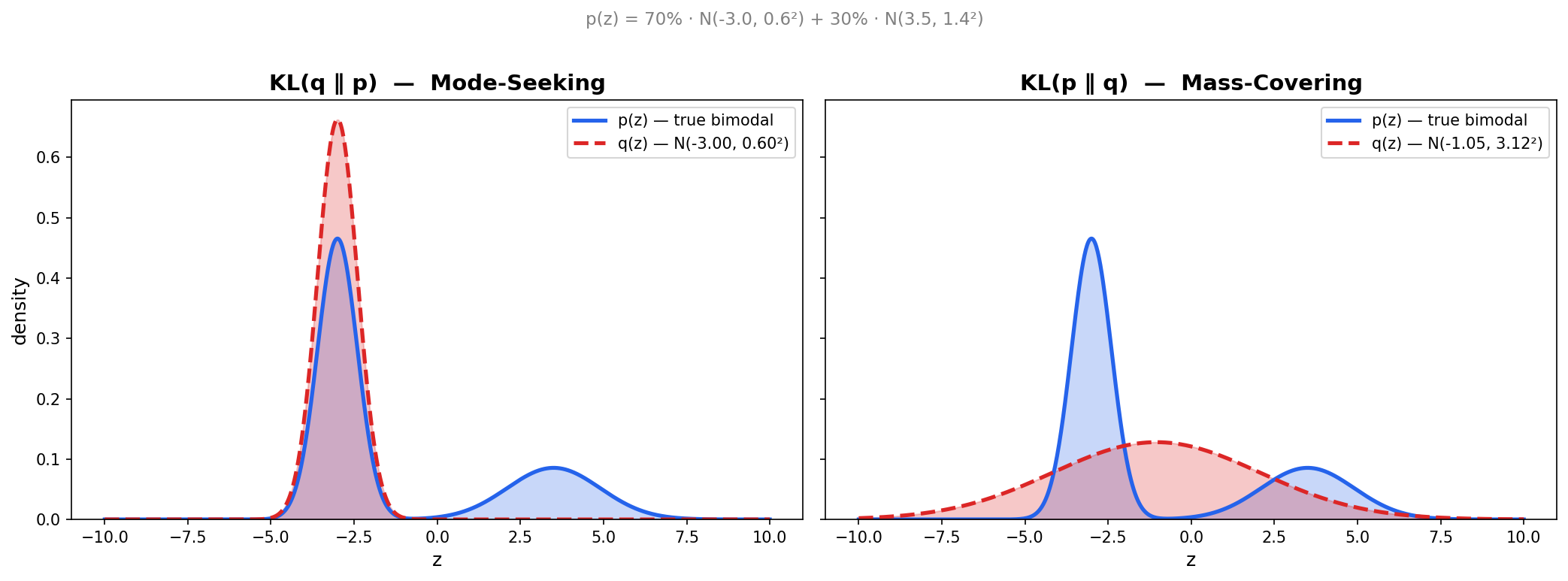
$D_{\mathrm{KL}}(q \parallel p)$ - mode-seeking

We’re taking the expectation under $q$ :

\[D_{\mathrm{KL}}(q \parallel p)=\mathbb{E}_q\left[\log \frac{q(z)}{p(z)}\right]\]

This blows up whenever $q(z)>0$ but $p(z) \approx 0$. So $q$ is severely penalized for putting mass where $p$ has none. The solution $q$ avoids any region where $p$ is small, and instead concentrates on a single mode of $p$ where it’s safe. If $p$ is bimodal, $q$ will pick one mode and ignore the other entirely rather than risk straddling the gap between them where $p$ is near zero.

$D_{\mathrm{KL}}(p \parallel q)$ - mass-covering

Now the expectation is under $p$ :

\[D_{\mathrm{KL}}(p \parallel q)=\mathbb{E}_p\left[\log \frac{p(z)}{q(z)}\right]\]

This blows up whenever $p(z)>0$ but $q(z) \approx 0$. So $q$ is penalized for missing any region where $p$ has mass. The solution $q$ spreads out to cover all modes of $p$. If $p$ is bimodal, $q$ will stretch itself wide enough to cover both modes, even if that means putting mass in the gap between them where $p$ is actually low.

The ELBO optimizes the mode-seeking direction $D_{\mathrm{KL}}\left(q_\phi(z \mid x) \parallel p_\theta(z \mid x)\right)$, which means the encoder will lock onto one mode of the true posterior if it’s multimodal.