Path equivalence, Holonomy and Single Tangent Fallacy

Part 5 of 5, following Part 1: Prior Knowledge, Part 2: The Group Structure of Neural Networks, Part 3: Path Equivariance, Part 4: A Category Theory Perspective

In this section we connect classical group equivariance, path equivariance (PE), holonomy, and the Single Tangent Space Fallacy [1]. We show that the holonomy group controls the expressivity of PE: when holonomy is trivial, PE reduces to classical group equivariance, the holonomy group captures exactly the information that group equivariance misses in curved spaces. We then use this framework to explain the Single Tangent Space Fallacy – why the single tangent space approach works on Lie groups but fails on general Riemannian manifolds. The group structure of a Lie group naturally ensures trivial holonomy, making path choice irrelevant; on a general Riemannian manifold, parallel transport is path-dependent, and collapsing to a single tangent space discards this information.

---

Classical Equivariant Neural Networks

Given a group $G$ acting on the data space $x \mapsto g \cdot x$ and simultaneously feature space $v \mapsto \rho(g) \cdot v$ , the classical equivariant neural networks enforce a global symmetry constraint, every layer $F$ satisfies

\[F \circ \rho(g) = \rho(g) \circ F \quad \forall\, g \in G\]

where $\rho : G \to GL(V)$ is a representation.

This works when the data space is homogeneous - $G$ acts transitively on this space. But many real data spaces are not homogeneous. A robot’s configuration space has regions of free motion and regions near joint limits. A molecular energy landscape has flat basins and sharp saddle points. Forcing the same symmetry everywhere is geometrically wrong: it respects symmetries that don’t exist in flat regions and fails to capture the path-dependence that curvature introduces.

The deeper issue is that features at different points live in different fibers (usually we use tangent space in manifold learning). A feature at $x \in M$ belongs to a fiber $E_x$, and a feature at $y$ belongs to $E_y$. There is no canonical way to compare them, we need a rule for moving vectors between fibers.

That is the reason we introduce path (or parallel transport) equivariance.

---

Path Equivariance (PE)

PE operates on an associated vector bundle $E = P \times_\rho V$ over a data manifold $M$, where $P \to M$ is a principal $G$-bundle and $\rho : G \to GL(V)$ is a representation. A feature at point $x$ is a vector $v \in E_x \cong V$.

A connection $\nabla$ on $P$ defines parallel transport along paths: given a path $\gamma : [0,1] \to M$, transport is a linear map

\[\tau_\gamma : E_{\gamma(0)} \to E_{\gamma(1)}\]

that slides vectors from one fiber to another. Crucially (which we will discuss later), $\tau_\gamma$ depends on the entire path $\gamma$, not just its endpoints $\gamma(0)$ and $\gamma(1)$, unless the connection is flat.

A PE layer $F$ acts pointwise: at each $x \in M$, there is a linear map $F_x : E_x \to E_x$. The defining constraint is

\[F_y \circ \tau_\gamma = \tau_\gamma \circ F_x\]

for every path $\gamma$ from $x$ to $y$.

In category theory language, we can draw the square commutes:

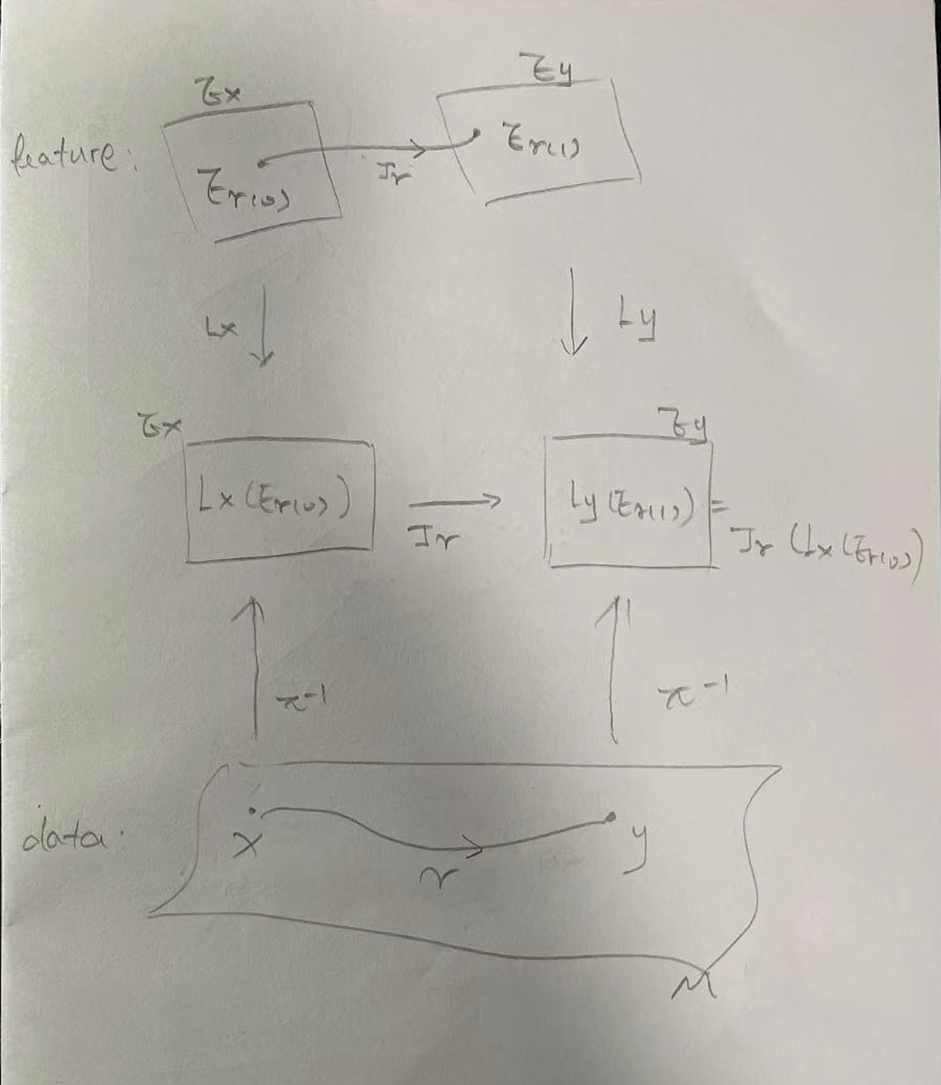
The parallel transport defines a functor $\tau : \mathcal{P}(M) \to \mathbf{Vect}$ , the layer $F$ which is a linear map $F_x : E_x \to E_x$ is a natural transformation from the functor $\tau$ to itself. The PEN constraint IS naturality.

Note: the $\pi^{-1}$ arrows connecting the data level to the feature level aren’t really a “map” in the usual sense — $\pi : E \to M$ is the bundle projection, and $\pi^{-1}(x) = E_x$ is the fiber. The fiber assignment is itself part of what the functor $\tau$ does.

The constraint is local and path-dependent. It does not require a global group action. It does not assume the data space is homogeneous. It asks only that the network respects the geometry encoded in the connection.

Holonomy Controls Expressivity

Now we need to ask a fundamental question about PEN: is transport path-dependent?

The PEN constraint applies to all paths, but not all paths are equally informative. For an open path $\gamma : x \to y$, the constraint $F_y \circ \tau_\gamma = \tau_\gamma \circ F_x$ couples two different maps at two different points. It tells us how $F_x$ and $F_y$ relate, but says nothing about what $F_x$ must commute with on its own.

Closed loops are different. When $\gamma$ starts and ends at $x$, the transport $\tau_\gamma : E_x \to E_x$ is an endomorphism of a single fiber, and the constraint collapses to $F_x \circ \tau_\gamma = \tau_\gamma \circ F_x$ - a commutation condition on $F_x$ alone. The holonomy group $\mathrm{Hol}x(\nabla)$ collects all such $\tau\gamma$ over every closed loop at $x$, so the PEN constraint on loops becomes

\[F_x \circ h = h \circ F_x \quad \forall\, h \in \mathrm{Hol}_x(\nabla)\]

This has the same algebraic form as global equivariance, but with $\mathrm{Hol}_x(\nabla)$ in place of $G$. Since $\mathrm{Hol}_x(\nabla) \subseteq G$, the constraint is generically weaker - the network has more freedom.

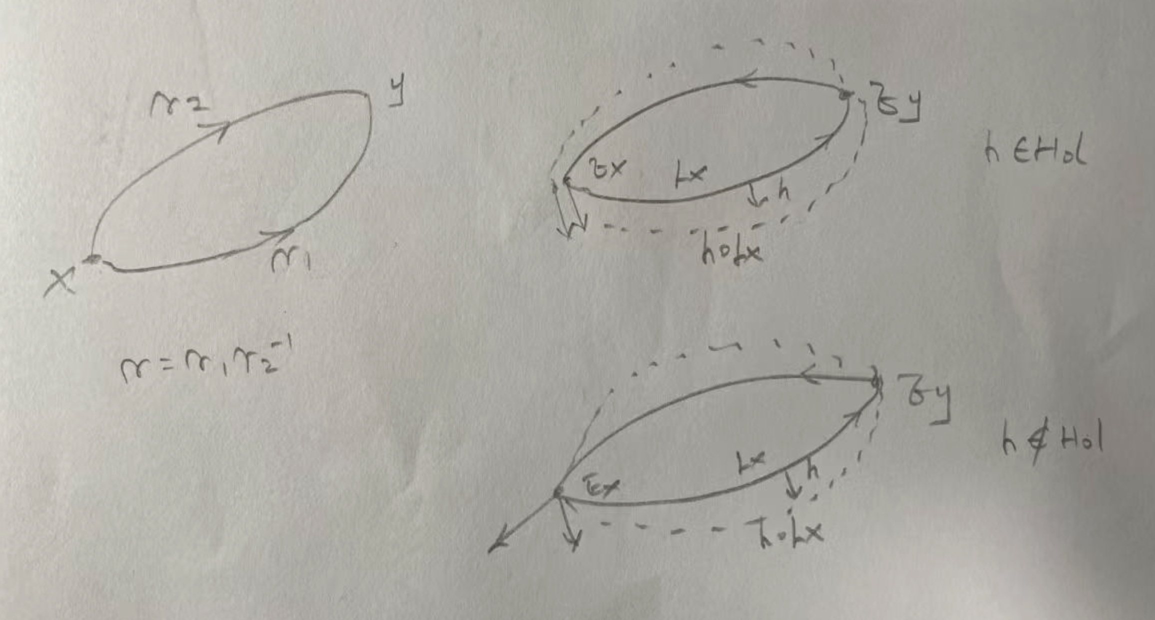
But why do loops at a single point tell us anything about transport between two different points? Because any two paths between the same endpoints compose into a loop. Take $\gamma_1, \gamma_2$ from $x$ to $y$ and form $\gamma = \gamma_1 \cdot \gamma_2^{-1}$. Its transport is

\[\tau_\gamma = \tau_{\gamma_2}^{-1} \circ \tau_{\gamma_1}\]

so $\tau_{\gamma_1} = \tau_{\gamma_2}$ if and only if $\tau_\gamma = \mathrm{id}$. Path-dependence between two points is detected by holonomy at one point.

Back to our question: is transport path-dependent? If every loop at $x$ gives trivial transport, then $\mathrm{Hol}_x(\nabla) = \lbrace e\rbrace$, transport is path-independent everywhere, and global equivariance suffices (PEN reduces to global equivariance). If some loop rotates a vector, different paths give different transports, and PEN is genuinely necessary.

The size of the holonomy group varies across the manifold, controlled by curvature. In flat regions where $\mathrm{Hol}_x$ is small, $F_x$ must commute with few elements and has high expressivity. In curved regions where $\mathrm{Hol}_x$ is large, $F_x$ must commute with many elements and is tightly constrained. PEN performs a spatially adaptive trade-off between expressive freedom and geometric fidelity, mediated by curvature through holonomy.

Reduction to Global Group Equivariance

(Path-Independent Condition) Given two paths $\gamma_1, \gamma_2$ from $x$ to $y$, we say the transport satisfies path-independent condition if

\[\tau_{\gamma_1}(v) = \tau_{\gamma_2}(v) \quad \forall v \in E_x\]

The destination vector depends only on where we start and where we end, not on how we get there.

On simply connected $M$, path-independence is equivalent to three other conditions, all describing the same phenomenon from different angles:

1. $\mathrm{Hol}(\nabla) = \lbrace e\rbrace$. Every closed loop transports vectors back to themselves. (trivial holonomy)
2. The connection is flat (zero curvature)
3. PEN collapses to classical equivariance: paths carry no more information than their endpoints

---

The Single Tangent Space Fallacy

This section draws on the paper Unraveling the Single Tangent Space Fallacy [1].

A common workaround for data on curved manifolds: pick a base point $p$, map everything to $T_pM$ via the logarithmic map $\mathrm{Log}_p$, and work in that single flat vector space. Geometrically, this imposes a flat connection on the tangent bundle - transport from any point to $p$ is the $\mathrm{Log}$ map, independent of path. The holonomy group is trivial: $\mathrm{Hol} = \lbrace e\rbrace$, the path-independent condition holds trivially, and PEN reduces to global equivariance. The cost is distortion. Points far from $p$ are mapped with increasing error, and the curvature information, which encodes genuine structure in the data, is discarded.

The tangent bundle approach keeps each point’s tangent space $T_xM$ separate. A vector at $x$ and a vector at $y$ live in different spaces, and comparing them requires parallel transport via the connection along a specific path. On a curved manifold this transport is path-dependent, holonomy is non-trivial, and PEN is the architecturally principled framework for respecting this structure.

The paper Unraveling the Single Tangent Space Fallacy makes the case concretely in robotics learning: the single-tangent-space approach is acceptable when the manifold is a Lie group, but introduces severe distortion on general Riemannian manifolds.

Lie Groups Case: It Is Fine

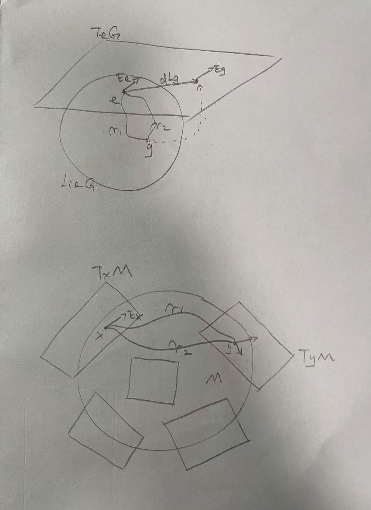
A Lie group $G$ acts on itself by left multiplication $L_g : h \mapsto gh$. Its differential $dL_g : T_eG \xrightarrow{\sim} T_gG$ canonically identifies every tangent space with the Lie algebra $\mathfrak{g} = T_eG$. There is no choice, no ambiguity, no path-dependence - the map is determined by $g$ alone. The connection is flat. The path-independent condition holds automatically: a path from $e$ to $g$ is fully characterized by $g$, and $f(g \cdot x) = \rho(g) \cdot f(x)$ works because $g$ encodes everything.

This is why the single tangent space approach is harmless on Lie groups — we’re not killing any holonomy, because there was none to begin with. The group structure of Lie group gives a unique identification between fibers (tangent space). The multiplication $e \mapsto g$ gives us $dL_g$ with no ambiguity, the parallel transport along any path from $e$ to $g$ agrees with $dL_g$.

Riemannian Manifolds Case: Why Fallacy

A general Riemannian manifold does not have group structure. There is no self-action and no canonical map between $T_xM$ and $T_yM$. We must specify a path $\gamma$ and use the Levi-Civita connection to transport. Different paths give different results. No single group element $g$ summarizes the relationship between $x$ and $y$, the path carries independent information. The classical equation $f(g \cdot x) = \rho(g) \cdot f(x)$ breaks down, and PEN becomes necessary.

Path-Independent Condition, Flat Mapping, and Group Representation

The path-independent condition says all paths with the same endpoints produce the same transport. When it holds, transport from $x$ to $y$ depends only on the pair $(x, y)$, not on the path. Pick a base point $x_0$: the transport $T(x_0, y) : E_{x_0} \to E_y$ is now well-defined for each $y$, and these transports compose consistently - $T(x_0, z) = T(y, z) \circ T(x_0, y)$ - so they form a group action on the fibers.

On a Lie group $G$, this is exactly what happens. The pair $(x, y)$ is captured by a single group element $xg = y$, the transport is a differential (pushforward) $dL_g$, and the path is redundant. The connection is flat, so the path-independent condition holds automatically and group equivariance is valid.

On a general curved Riemannian manifold, the transport $T(x, y)$ is not well-defined - it depends on the route. No single group element summarizes the relationship between $x$ and $y$, and standard group equivariance breaks down.

On simply connected $M$, the following conditions are equivalent:

1. The connection is flat.
2. $\mathrm{Hol}(\nabla) = \lbrace e\rbrace$. Every closed loop transports vectors back to themselves.
3. PEN collapses to classical equivariance: paths carry no more information than their endpoints.
4. Transport is path-independent: $\tau_{\gamma_1} = \tau_{\gamma_2}$ for all paths sharing the same endpoints.
5. Transport defines a consistent group action on fibers: $T(x, y) : E_x \to E_y$ depends only on $(x, y)$, and these maps compose as a group.

When any of these fails, the connection is curved, transport is path-dependent, no consistent group action exists, and PEN is necessary.

One important distinction: flatness here is a property of the connection on the bundle, not of the base space. The manifold itself can be curved, e.g.$SO(3)$ is not flat as a Riemannian manifold, yet can still carry a flat connection on its tangent bundle . The geometry of the base space and the geometry of the connection are independent.

Summary

In classical equivariance, a path from $e$ to $g$ is summarized by the group element $g$ - the path is redundant, and the equivariance condition $f(g \cdot x) = \rho(g) \cdot f(x)$ mentions only $g$. In PEN, the path $\gamma$ itself is the fundamental object. The equivariance condition

\[F_y \circ \tau_\gamma = \tau_\gamma \circ F_x\]

is indexed by paths, not group elements. The parallel transport $\tau_\gamma$ plays the role that $g$ played in classical equivariance, but depends on the entire path, not just its endpoints. This is a genuine generalization: when the connection is flat, $\tau_\gamma$ depends only on endpoints, paths collapse to group elements, and PEN recovers classical equivariance. When the connection is curved, $\tau_\gamma$ carries strictly more information, and the path is irreplaceable.

The holonomy group $\mathrm{Hol}(\nabla)$ measures the gap between these regimes. Trivial holonomy means group equivariance suffices. Non-trivial holonomy means it doesn’t - and PEN provides a spatially adaptive inductive bias, constrained where curvature demands it, expressive where geometry permits it.

---

Spherical Cow in a Vacuum

The theoretical framework is clean. The practical question is harder: where does the connection come from? With group equivariance, the workflow is straightforward : domain knowledge gives us the symmetry group, and we build layers that respect it. With PEN, the connection is not typically known in advance.

• Connection known. The data lives on a manifold with a known Riemannian metric e.g. robot arms, molecular dynamics, general relativity. The Levi-Civita connection is determined, parallel transport can be computed analytically, and PEN layers commute with it exactly. This might be the cleanest case.

• Connection constrained. The manifold $M$ is known (e.g., SPD matrices, a Lie group quotient), but there is a family of possible connections. Domain knowledge constrains the holonomy group to a subgroup of $G$. PEN provides the architectural scaffold; the specific connection is selected or learned within the constrained family.

• Connection learned. The data manifold itself is unknown. The manifold, the bundle, and the connection are learned jointly. This is the most ambitious regime. PEN provides an inductive bias: whatever connection the network learns, the layers automatically respect its parallel transport.

What PEN buys over group equivariance

Group equivariance imposes the same symmetry constraint everywhere, it assumes the data space is homogeneous. Many real spaces are not. A robot arm near a joint limit is highly curved and constrained; far from joint limits, it is nearly flat and free. A globally equivariant network cannot adapt to this variation. PEN can, because the holonomy constraint automatically tightens where curvature is high and loosens where it is low. The result is a spatially adaptive inductive bias instead of a uniform one.

---

Reference

[1] Jaquier, N., Rozo, L., & Asfour, T. (2024). Unraveling the Single Tangent Space Fallacy: An Analysis and Clarification for Applying Riemannian Geometry in Robot Learning. arXiv preprint arXiv:2310.07902. https://arxiv.org/abs/2310.07902