Part2-GroupStructure
The group structure: a type of formalized prior knowledge
Part 2 of 5, following Part 1: Prior Knowledge
Code can be found in https://github.com/bozh3ng/ThesisExp part2_group_structure.
In the previous article, I argued that every component of a neural network encodes prior knowledge, and that this knowledge can be formalized as the restriction of symmetry. Here we make that claim concrete. Using group theory, we trace the symmetry of a deep network from its maximally redundant starting point which is the deep linear network. The redundancy is then successively reduced by activation functions and regularization.
The results are surprisingly clean. Each component maps to a specific subgroup of the general linear group, and the hierarchy of these subgroups tells a coherent story about what the network “knows” before training.
Starting point: the deep linear network
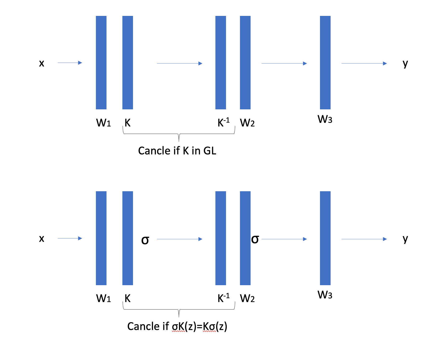
A deep linear network with $L$ layers computes $f(x) = W^{(L)} \cdots W^{(1)} x$. Only the product $W_{\text{total}} = \prod_\ell W^{(\ell)}$ matters for the input-output function; the individual factors are interchangeable. Concretely, for any invertible matrix $K \in \mathrm{GL}(n_\ell)$ at hidden layer $\ell$, we can insert $K$ after one layer and $K^{-1}$ before the next without changing the function.
The full symmetry group is $\mathcal{G} = \prod_{\ell=1}^{L-1} \mathrm{GL}(n_\ell)$.
This is a massive group. Each realized linear map $W_{\text{total}}$ corresponds to an entire orbit of parameter configurations: an infinite family of weight matrices that all compute the same function. In machine learning terms, the map from parameter space $\mathcal{P}$ to hypothesis space $\mathcal{H}$ is wildly non-injective. The fibers $\Phi^{-1}(W_{\text{total}})$ are exactly these orbits.
The takeaway: a deep linear network carries almost no prior knowledge. It assumes only linearity and imposes no further structure on how the linear map should be factored across layers.
Why this matters: the reparametrization problem
This symmetry is not an abstract curiosity. It is the reparametrization problem, formalized. Nobody deliberately inserts $K$ and $K^{-1}$ between layers. The point is that this redundancy already exists. If we train a network and arrive at weights $\left(W_1, W_2, W_3\right)$, then $\left(K W_1, W_2 K^{-1}, W_3\right)$ computes the exact same function for every invertible $K$ : the data flows as
\[x \rightarrow K W_1 x \rightarrow W_2 K^{-1}\left(K W_1 x\right)=W_2 W_1 x \rightarrow W_3 W_2 W_1 x\]The $K$ and $K^{-1}$ cancel between adjacent layers. These are different points in parameter space that gradient descent treats as distinct, even though they are functionally identical.
This has real consequences. The loss function is constant along orbits of the symmetry group, flat valleys corresponding to movement within an orbit. A large symmetry group means a large fraction of the parameter space is redundant. Gradient descent can waste capacity wandering between equivalent solutions and interpreting learned weights becomes ambiguous: which point on the orbit is the “true” representation?
The group-theoretic framework gives this problem precise structure. The set of all equivalent reparametrizations is the symmetry group $\mathcal{G}$. The set of all parameter configurations equivalent to a given one is its orbit under $\mathcal{G}$. The “true” space of distinct functions is the quotient $\mathcal{P}/\mathcal{G}$. And as we will see, each design choice (activation, regularization, architecture) shrinks $\mathcal{G}$, reducing the ambiguity and resolving the reparametrization problem step by step.
Remark (orbit size and expressivity). There is a precise geometric relationship between symmetry and expressivity. When $\mathcal{G}$ is large, orbits are large: many parameter configurations collapse to the same function, so the quotient $\mathcal{P}/\mathcal{G}$ is small and few distinct functions are representable. When activation functions shrink $\mathcal{G}$, orbits become smaller, and the same parameter space gets partitioned into more equivalence classes. The quotient grows. More distinct functions emerge, not because something was added, but because the symmetry that was hiding their distinctness has been removed.
Note that this is a different sense of “constraint” from the prior knowledge discussed in Part 1. The $\mathrm{GL}(n)$ symmetry of a linear network constrains the parameter space: it forces massive redundancy, collapsing the function class to linear maps. Breaking this symmetry via activation releases expressivity. By contrast, architectural priors like translation equivariance constrain the function class: they restrict which functions are representable, shrinking the search space to a useful subspace. The full design of a network involves both moves: break enough parameter-space symmetry to have a rich function class, then constrain that class to match the problem.
Remark (orbit flatness vs. functional flatness). The flat valleys created by the symmetry group $\mathcal{G}$ should not be confused with the “flat minima” that the generalization literature associates with good test performance. These are flatness in orthogonal senses. Orbit flatness is movement within a fiber $\Phi^{-1}(h)$: the parameters change, but the realized function $h \in \mathcal{H}$ does not, and the loss is exactly constant. This is redundancy — it inflates the parameter space without expanding the function class. Functional flatness is movement that changes the function: nearby but distinct $h’ \neq h$ also achieve low loss, so the solution is robust to the distribution shift between training and test data. The former lives in the kernel of the map $\Phi: \mathcal{P} \to \mathcal{H}$; the latter lives in its complement.
This distinction has a concrete consequence: naive flatness measures in $\mathcal{P}$ conflate the two. (Dinh et al. Sharp Minima Can Generalize For Deep Nets 2017) demonstrated this directly for ReLU networks. Using the positive scaling symmetry $\mathcal{D}^+$ — the same residual group identified above — they showed that any minimum can be reparametrized to have arbitrarily large or small Hessian eigenvalues. Scale one layer’s weights by $\alpha > 0$ and the adjacent layer’s by $1/\alpha$; the function is unchanged (it is an orbit move under $\mathcal{D}^+$), but the curvature in parameter space scales as $\alpha^2$. Sharp minima can be made to look flat and vice versa, without affecting generalization. Raw flatness in $\mathcal{P}$ is a gauge artifact, not a geometric invariant.
The group-theoretic framework resolves this: the meaningful geometry lives on the quotient $\mathcal{P}/\mathcal{G}$, where orbit directions are factored out. Flatness in the quotient — functional flatness — is invariant under reparametrization and is the quantity relevant to generalization. Each design choice that shrinks $\mathcal{G}$ (activation, regularization) reduces the gap between $\mathcal{P}$ and $\mathcal{P}/\mathcal{G}$, making parameter-space measurements more faithful to the true functional geometry.
Activation functions break symmetry
Now introduce a nonlinear activation $\sigma$ between layers. The reparametrization trick, inserting $K$ and $K^{-1}$, no longer works for arbitrary $K$, because $\sigma$ gets in the way. Only those $M$ that commute with $\sigma$ still leave the network function unchanged.
This surviving symmetry is the centralizer of the activation:
\[\mathrm{Cent}(\sigma) = \lbrace K \in \mathrm{GL}(n) : \sigma(Kz) = K\sigma(z) \text{ for all } z\rbrace\]Different activations yield dramatically different centralizers.
ReLU
For the element-wise ReLU $\sigma(z) = \max(0, z)$, the centralizer is:
\[\mathrm{Cent}(\mathrm{ReLU}) \cong \mathcal{D}^+ \rtimes S_n\]where $\mathcal{D}^+$ is the group of diagonal matrices with strictly positive entries and $S_n$ is the symmetric group (all permutations).
The intuition is direct. ReLU acts coordinate-wise and only cares whether each component is positive or negative. Permuting coordinates before or after ReLU makes no difference, and that accounts for the $S_n$ part. Scaling a coordinate by a positive factor also commutes: $\mathrm{ReLU}(\alpha z_i) = \alpha \cdot \mathrm{ReLU}(z_i)$ when $\alpha > 0$. But negative scaling breaks it: $\mathrm{ReLU}(-z_i) \neq -\mathrm{ReLU}(z_i)$ whenever $z_i \neq 0$. ReLU distinguishes positive from negative, and this asymmetry is precisely what shatters the full $\mathrm{GL}(n)$ symmetry.
What this means for the network: in a ReLU network, the identity of each neuron is determined only up to positive rescaling and reordering. Two parameter configurations related by such a map compute exactly the same function. Any other reparametrization changes the network’s behavior.
Sigmoid
For the element-wise sigmoid $\sigma(z) = 1/(1+e^{-z})$, the centralizer shrinks to:
\[\mathrm{Cent}(\mathrm{sigmoid}) = S_n\]Only permutations survive. No rescaling commutes with sigmoid, not even positive scaling, because sigmoid’s nonlinear compression of the real line means $\sigma(\alpha z) \neq \alpha \sigma(z)$ for any $\alpha \neq 1$.
Sigmoid thus encodes a stronger prior than ReLU. It breaks more symmetry, leaving only the discrete freedom of reordering neurons.
The hierarchy
This gives a strict chain of subgroups:
\[S_n \;\subsetneq\; \mathcal{D}^+ \rtimes S_n \;\subsetneq\; \mathrm{GL}(n)\] \[\text{(sigmoid)} \qquad\quad \text{(ReLU)} \qquad\quad \text{(linear)}\]More symmetry broken means fewer equivalent parametrizations, which means a stronger structural commitment. The price of ReLU’s extra symmetry (positive rescaling freedom) is a form of under-determination that sigmoid avoids; the benefit is a simpler loss surface with more equivalent paths to each function.
Remark (why more residual symmetry can help training). The subgroup chain $S_n \subsetneq \mathcal{D}^+ \rtimes S_n \subsetneq \mathrm{GL}(n)$ might suggest sigmoid is the “strongest” choice, having the smallest residual group. In practice, ReLU wins often. The group perspective offers a partial explanation: ReLU’s larger residual symmetry means more equivalent parametrizations per function, which means more paths through parameter space reach the same solution. The loss surface has more highways to good minima. Sigmoid’s smaller group makes things more rigid, with fewer routes to each solution. The practical sweet spot is not maximum symmetry breaking but the right balance: enough broken for universal approximation, enough remaining for gradient descent to move efficiently. Other factors (vanishing gradients, computational cost, activation sparsity) also contribute to ReLU’s dominance, but the symmetry view captures a genuine geometric piece of the story.
A connection to universal approximation
This hierarchy suggests something deeper: the link between symmetry reduction and the universal approximation theorem (UAT) is not merely descriptive but structural. The deep linear network has maximal symmetry ($\mathrm{GL}(n)$) and can only express linear functions. The moment any activation breaks $\mathrm{GL}(n)$ to a proper subgroup, whether it is ReLU’s $\mathcal{D}^+ \rtimes S_n$ or sigmoid’s $S_n$, expressivity jumps to universal approximation. The specific residual group barely matters for this qualitative leap; what matters is that $\mathrm{GL}(n)$ is broken. It is a phase transition: full symmetry means linear, any proper subgroup means universal.
Why should this be the case? The $\mathrm{GL}(n)$ symmetry forces the network to be linear. The function must be invariant under arbitrary invertible reparametrizations of hidden layers, and this constraint collapses the function class. Breaking the symmetry lifts this constraint, and each nonlinear layer introduces a “fold” in the network’s image within function space. Depth compounds these folds, giving exponential growth in the topological complexity of the set of representable functions.
There is likely a purely topological proof of UAT along these lines: iterated nonlinear folding generates enough topological complexity in the image of the network map $\Phi: \mathcal{P} \to C(X, \mathbb{R})$ to make that image dense. The classical proofs use analysis (Stone–Weierstrass, step-function constructions); a topological proof would instead argue via the structure of the image manifold, its local dimension, its degree, or its homotopy type. This remains an open direction, but the symmetry-breaking framework points squarely at it: UAT is what happens when we break enough symmetry to allow topologically nontrivial maps into function space.
Regularization: choosing representatives within orbits
Activation functions reduce the reparametrization ambiguity but don’t eliminate it. Even after introducing ReLU, the network still has a large family of equivalent parametrizations (the $\mathcal{D}^+ \rtimes S_n$ orbits). The model may still suffer from an excess-of-choices problem. Regularization addresses this further: it breaks the remaining symmetry by penalizing some orbit members over others, effectively selecting a preferred representative from each equivalence class.
To analyze this cleanly, consider a linear autoencoder (encoder $f(x) = Wx$, decoder $g(h) = W’h$) where the latent-space symmetry is the full $\mathrm{GL}_d(\mathbb{R})$. Any invertible $K$ can be inserted between encoder and decoder ($W \mapsto KW$, $W’ \mapsto W’K^{-1}$) without changing the reconstruction $W’Wx$. Different regularizers break this symmetry to different subgroups.
The general framework: Jacobian-based regularization
We study the general loss:
\[\mathcal{L}(f, g) = \sum_{x} \left[ L(x, g(f(x))) + \lambda_E\lVert J_f(x)\rVert_E + \lambda_D\lVert J_g(f(x))\rVert_D \right]\]where $\lVert \cdot\rVert_E$ and $\lVert \cdot\rVert_D$ are matrix norms on the encoder and decoder Jacobians. Under the map $K$, the Jacobians become $J_{f’} = KJ_f$ and $J_{g’} = J_g K^{-1}$. The residual symmetry group is determined by which $K$ leave both norm terms unchanged, the intersection of the left-isometry group of $\lVert \cdot\rVert_E$ and the right-isometry group of $\lVert \cdot\rVert_D$.
The question thus reduces to: for which invertible $K$ does
\[\lVert K A\rVert_p=\lVert A\rVert_p\]hold for every matrix $A$ ? That is, which linear maps are isometries of the matrix norm $\lVert \cdot\rVert_p$ ? The answer depends on the geometry of the norm’s unit ball, and this is where the choice of norm becomes decisive.
Frobenius / Schatten-$p$ norms → orthogonal group
When the regularization uses any unitarily invariant norm (norms that depend only on the singular values of the matrix, including the Frobenius norm as the case $p=2$), the residual symmetry group is:
\[\mathcal{G} = O_d(\mathbb{R})\]The regularizer treats all orthogonal reparametrizations as equally costly but penalizes non-orthogonal ones. In concrete terms: rotating the latent space is free, but shearing or scaling it is not. The prior knowledge here is that the natural geometry of the latent representation is Euclidean. Distances and angles between encoded features matter, but the choice of orthonormal basis does not.
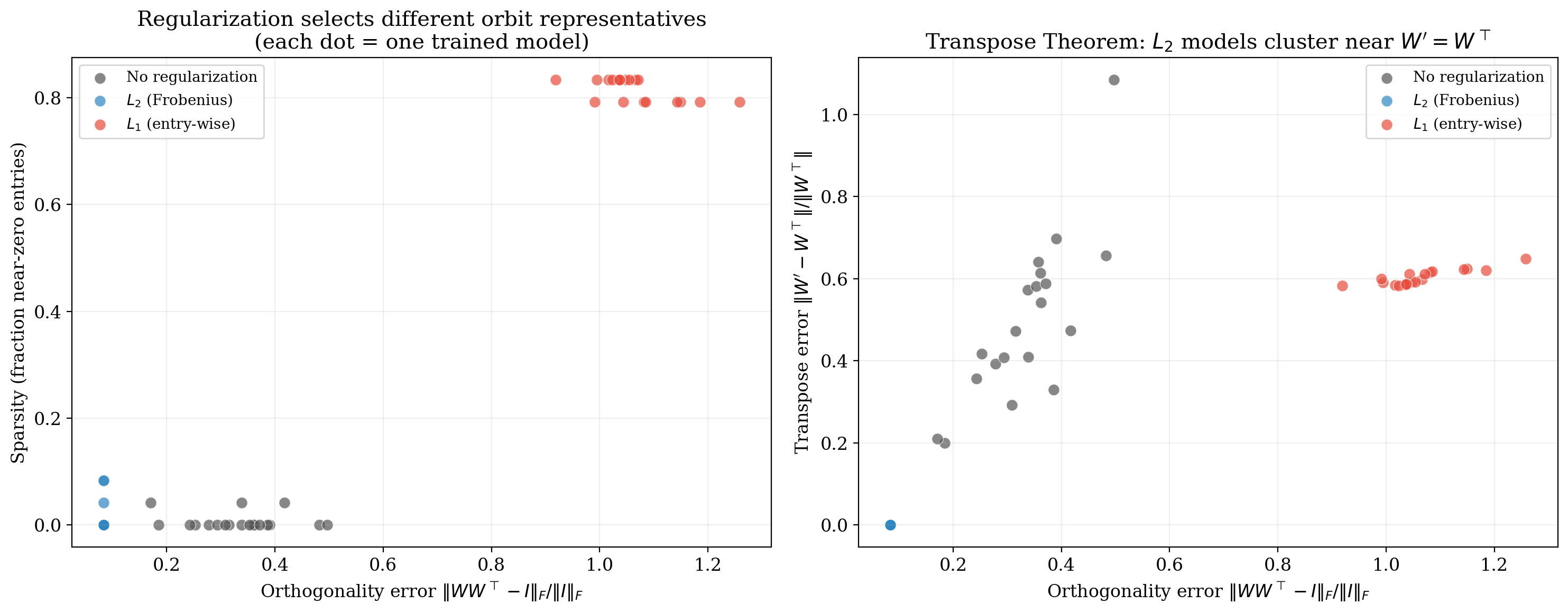
This explains a classical result: all critical points of $L_2$-regularized linear autoencoders satisfy $W’ = W^\top$ (the Transpose Theorem of Kunin et al., 2019). Tied weights are not just a computational convenience; they are the natural consequence of the orthogonal symmetry that $L_2$ regularization imposes.
Entry-wise $\ell_p$ norms ($p \neq 2$) → hyperoctahedral group
When regularization uses the entry-wise $\ell_p$ norm with $p \neq 2$, the picture changes dramatically. A classical result in functional analysis (the Banach–Lamperti theorem) states that the only linear operators preserving the $\ell_p$ norm for $p \neq 2$ are signed permutation matrices. This forces the residual symmetry down to:
\[\mathcal{G} = B_d \cong \mathbb{Z}_2^d \rtimes S_d\]the hyperoctahedral group, coordinate permutations composed with sign flips. This is a finite group with $2^d \cdot d!$ elements, compared to the infinite-dimensional $O_d(\mathbb{R})$.
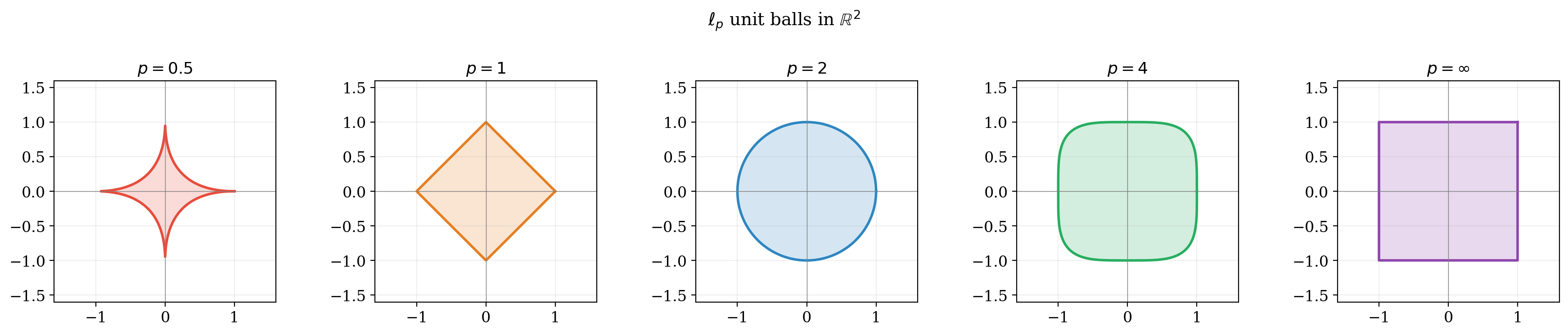
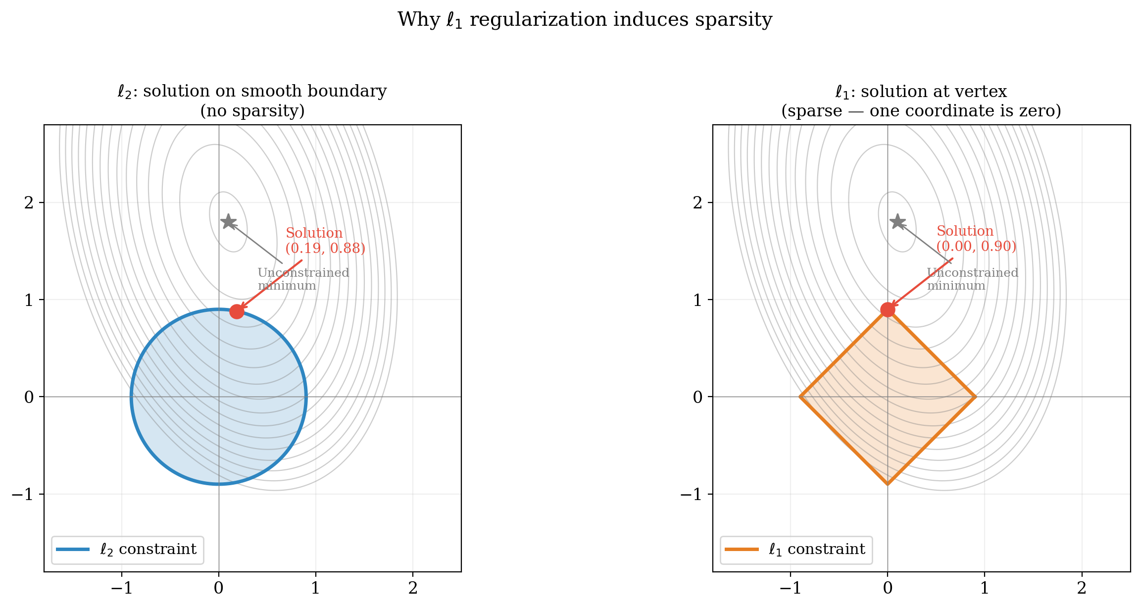
The geometric picture here is worth pausing on. The $\ell_2$ unit ball is a sphere: continuous rotational symmetry, no preferred direction. The $\ell_1$ unit ball is a cross-polytope (a diamond) whose only symmetries are reflections and permutations of the coordinate axes. The diamond has corners sitting on the coordinate axes, and when smooth loss contours meet a shape with corners, the contact point is generically at a vertex, right on an axis. This is where the sparsity prior actually comes from. The symmetry groups summarize this neatly: $O_d(\mathbb{R})$ says no direction is special; $B_d$ says only the coordinate axes are. There is a classical visualization.
How do these sphere and diamond become groups? The residual symmetry of regularization reduces to the question: which linear maps send the $\ell_p$ unit ball to itself? For $p=2$, the ball is a sphere, and any rotation or reflection preserves it: giving $O_d(\mathbb{R})$. For $p \neq 2$, the ball has corners at $\pm e_i$ (the standard basis vectors), and a linear isometry must map corners to corners. The only such maps are permutations of the axes and sign flips giving the hyperoctahedral group $B_d$. The Banach-Lamperti theorem is the rigorous version of this geometric observation: the shape of the unit ball determines its isometry group, and that isometry group is the residual symmetry of the regularization.
Summary table
| Regularization | Residual group | Size | Type |
|---|---|---|---|
| Frobenius / Schatten-$p$ | $O_d(\mathbb{R})$ | $\infty$ | Continuous (Lie group) |
| Entry-wise $\ell_p$, $p \neq 2$ | $B_d$ | $2^d \cdot d!$ | Discrete (finite) |
| None | $\mathrm{GL}_d(\mathbb{R})$ | $\infty$ | Continuous (non-compact) |
The scaling loophole
One subtlety deserves mention. When encoder and decoder weights are independent, a positive scalar $\alpha$ can be absorbed: $W \mapsto \alpha W$, $W’ \mapsto \frac{1}{\alpha} W’$. This preserves reconstruction but changes regularization asymmetrically, allowing the network to shift complexity between encoder and decoder. Contractive autoencoders address this by tying weights ($W’ = W^\top$), which pins $\alpha = 1$ and closes the loophole. This is not an ad hoc fix; it is the natural response to a residual symmetry that the regularizer alone fails to break.
Experiments
The theory above makes precise claims: the loss is constant along orbits, activation functions break $\mathrm{GL}(n)$ to specific subgroups, regularization selects preferred representatives. We verify these claims on small networks where the full structure is computable.
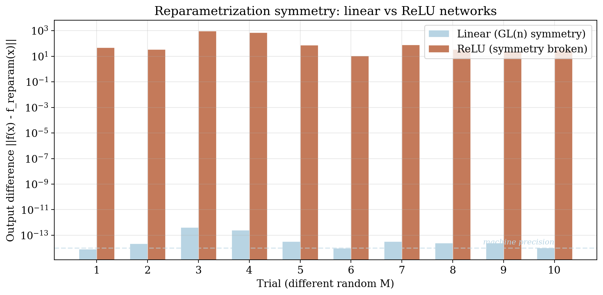
Experiment 1: Reparametrization symmetry
We train a 3-layer deep linear network $f(x) = W_3 W_2 W_1 x$ and verify that inserting $K$ and $K^{-1}$ between layers leaves the function unchanged. For 1000 random invertible matrices $K$, the reparametrized weights $(KW_1, W_2 K^{-1}, W_3)$ produce identical outputs to machine precision, confirming that $\mathrm{GL}(n)$ is an exact symmetry.
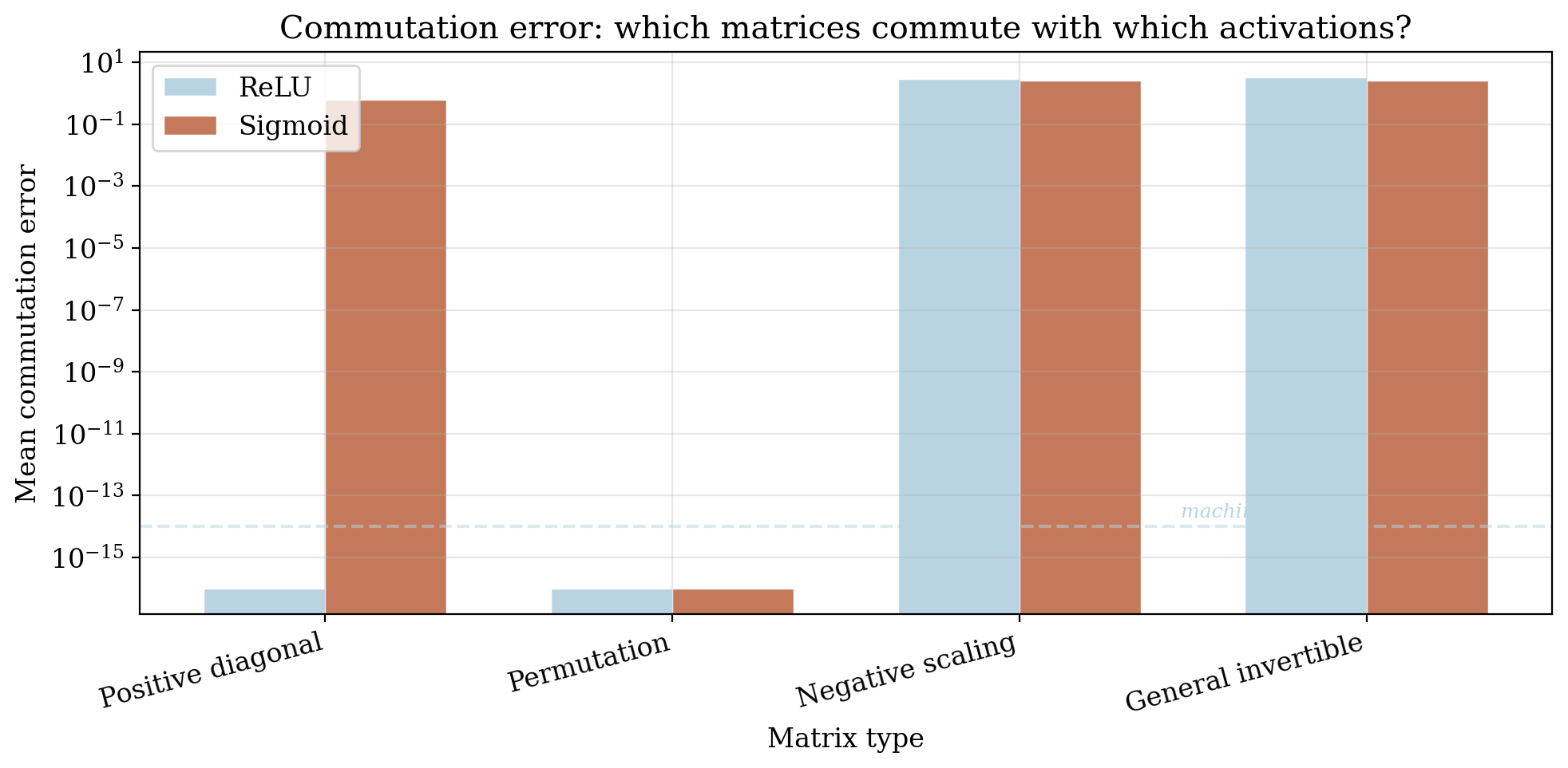
Experiment 2: Activation centralizers
We test which reparametrizations survive different activation functions. For each candidate $K$, we check whether $\sigma(Kz) = K\sigma(z)$ holds for random inputs. The results confirm the predicted centralizer hierarchy: all of $\mathrm{GL}(n)$ survives for linear activations, only $\mathcal{D}^+ \rtimes S_n$ for ReLU, and only $S_n$ for sigmoid/tanh.
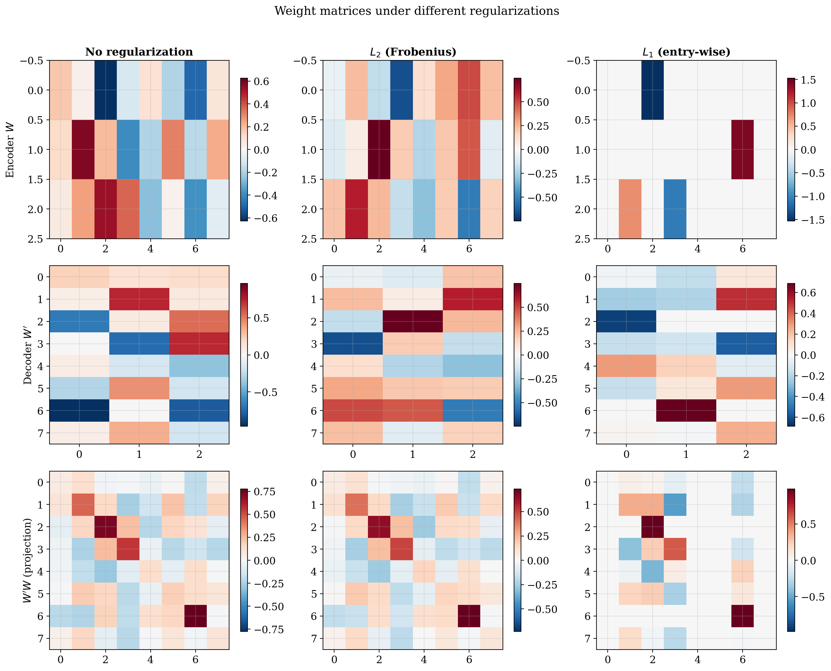
Experiment 3: Regularization geometry
We train linear autoencoders under three regimes (no regularization, $\ell_2$, and $\ell_1$) and examine the learned weight structure.
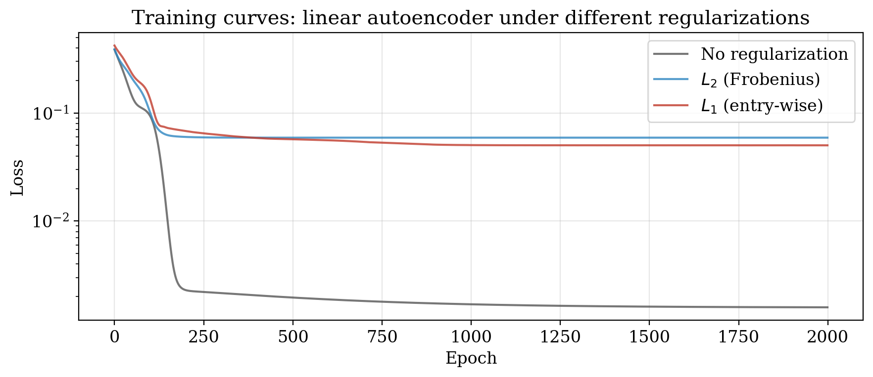
The weight matrices confirm the prediction. Under $\ell_2$, $W’ \approx W^\top$ (the Transpose Theorem), reflecting orthogonal symmetry. Under $\ell_1$, the weights are sparse, reflecting the hyperoctahedral symmetry that privileges coordinate axes.
A multi-seed scatter plot makes this quantitative. Each dot is one trained model. $\ell_2$ models cluster at high orthogonality and zero sparsity; $\ell_1$ models cluster at high sparsity; unregularized models sit at the origin.
Experiment 4: Unit ball geometry
The residual symmetry of a regularizer reduces to: which linear maps send the $\ell_p$ unit ball to itself? The $\ell_2$ ball is a sphere with continuous rotational symmetry; the $\ell_1$ ball is a cross-polytope with only signed permutation symmetry.
Applying transformations confirms: rotations preserve the $\ell_2$ ball but distort the $\ell_1$ ball; signed permutations preserve both.
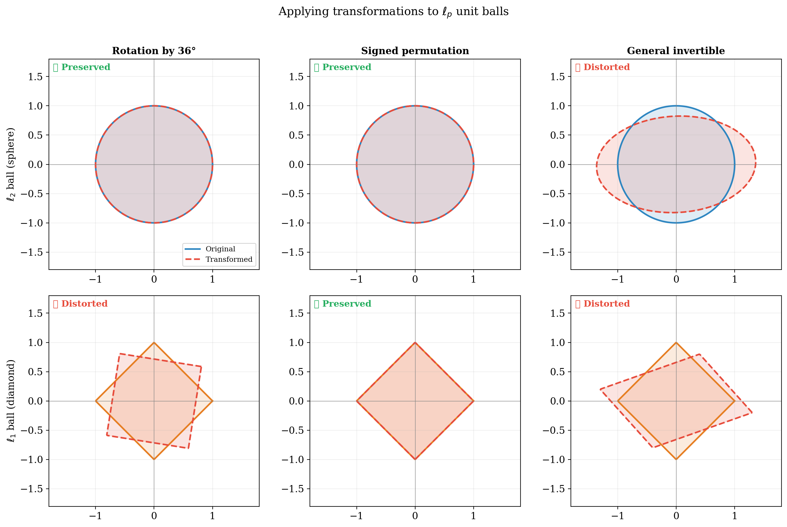
The geometric reason $\ell_1$ induces sparsity: constrained optimization on the cross-polytope generically lands at a vertex (where coordinates are zero), while on the sphere it lands on a smooth boundary point.
Experiment 5: Orbit structure and the loss landscape
Using $K(t) = e^{tA}$ to parametrize movement along the orbit, we confirm the loss is exactly constant in the orbit direction while it varies rapidly perpendicular to it.
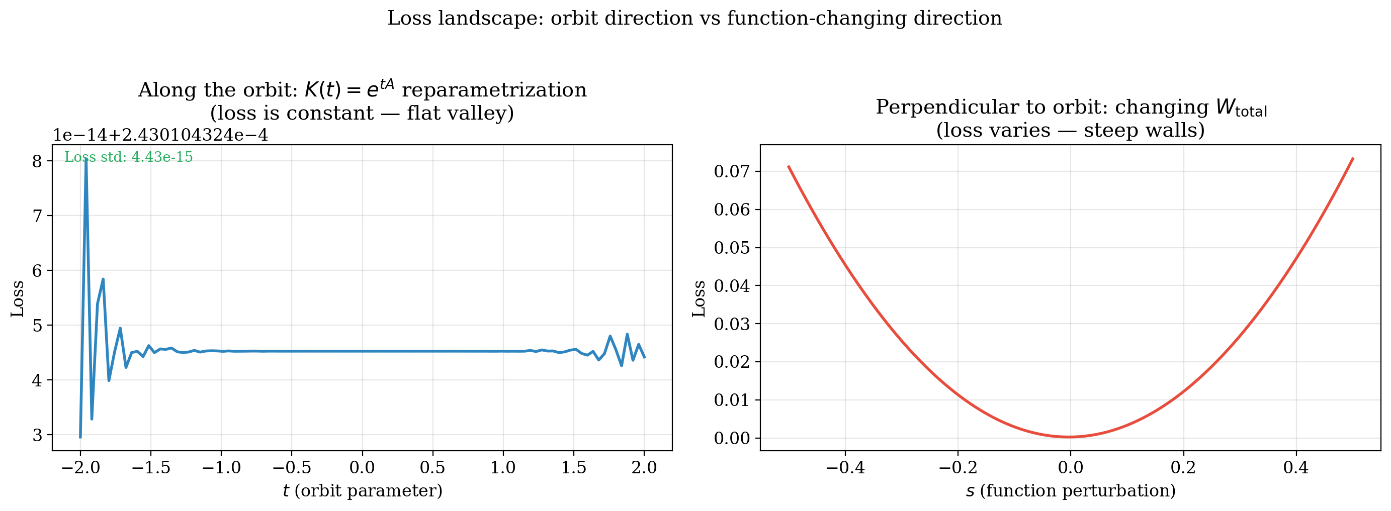
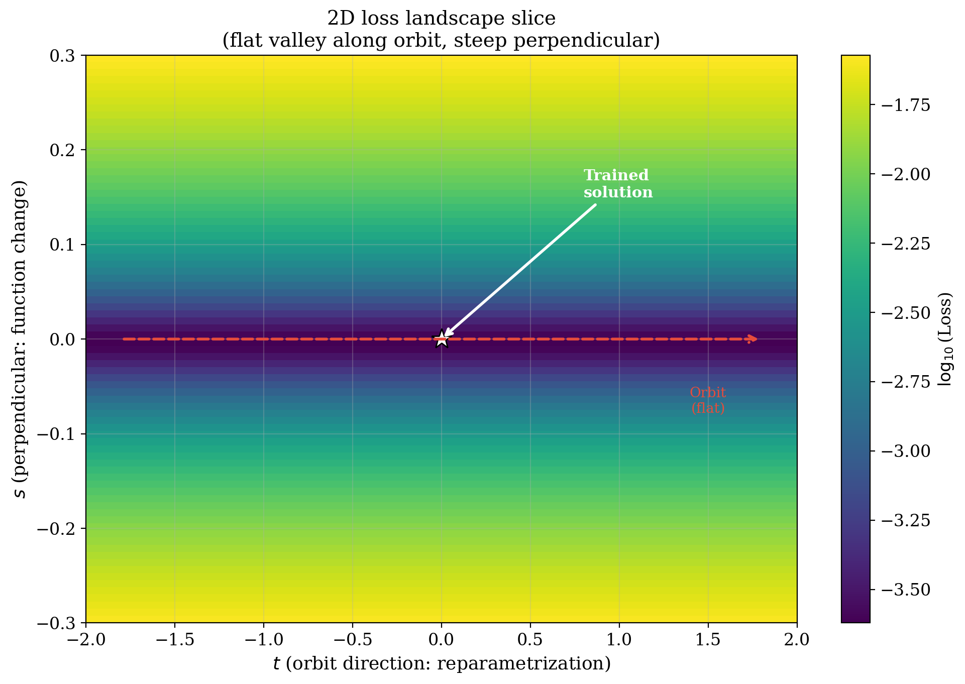
A 2D slice reveals the geometry: a flat valley along the orbit direction with steep walls perpendicular to it.
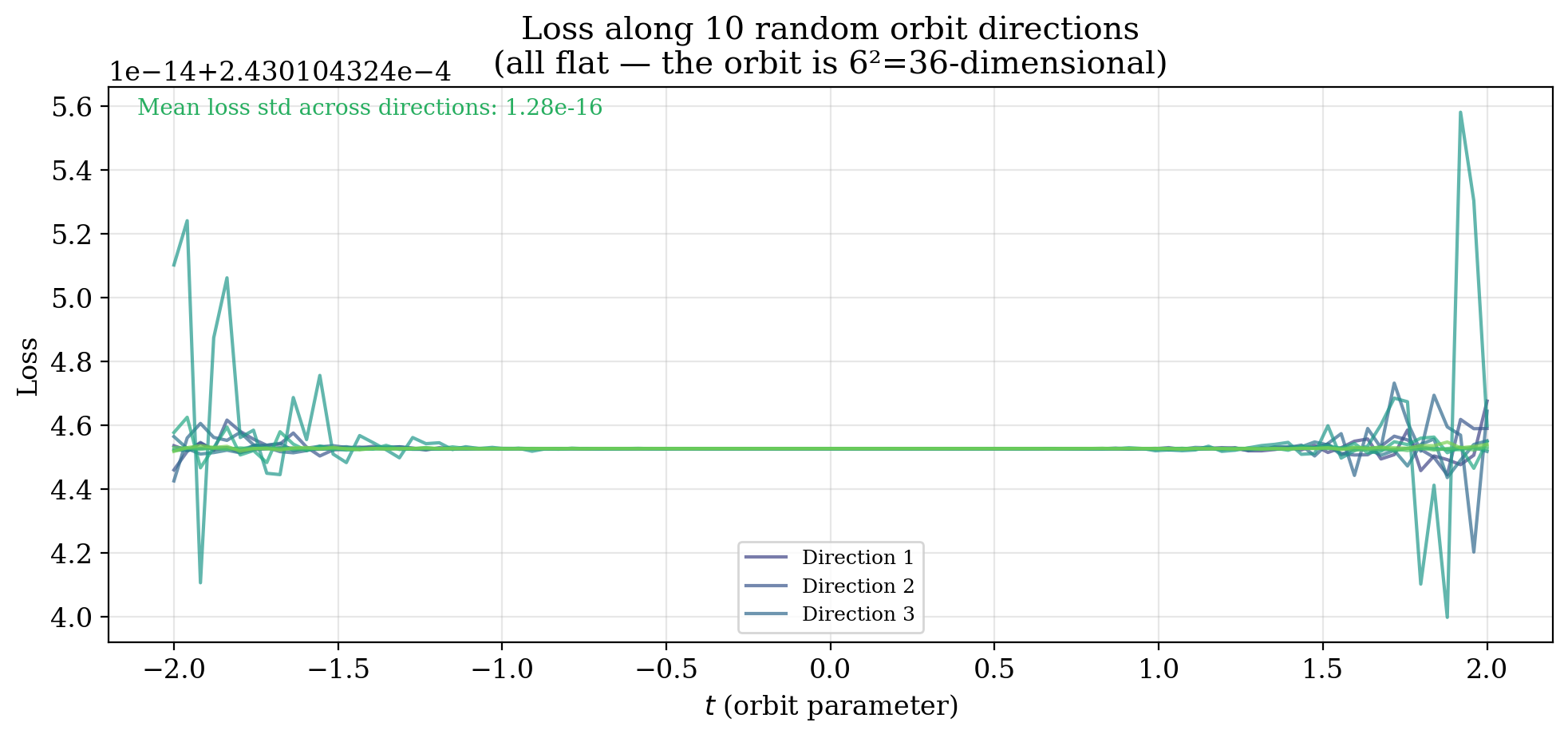
The orbit is not one-dimensional but $n^2$-dimensional. We verify flatness along 10 independently sampled orbit directions.
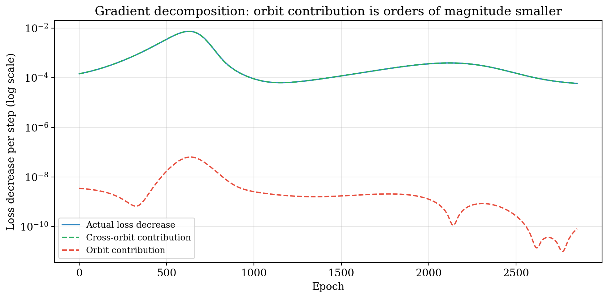
Finally, we decompose the gradient into orbit and cross-orbit components by projecting onto the orbit tangent space $T_\text{orbit} = \lbrace(AW_1, -W_2 A) : A \in \mathfrak{gl}(n)\rbrace$ via least-squares. The cross-orbit component accounts for all loss reduction ($\sim 10^{-4}$); the orbit component contributes nothing ($\sim 10^{-9}$). The gradient is orthogonal to the orbit, as it must be.
The full picture
Assembling these results, the design of a neural network traces a path through a hierarchy of groups:
\[\mathrm{GL}(n) \;\xrightarrow{\text{activation}}\; \mathrm{Cent}(\sigma) \;\xrightarrow{\text{regularization}}\; G_{\text{reg}}\]Each arrow injects prior knowledge, and each arrow is a step toward resolving the reparametrization problem. The deep linear network starts with maximal ambiguity: an enormous $\mathrm{GL}(n)$ family of equivalent parametrizations. Activation functions collapse most of this redundancy. Regularization collapses more. The residual group tells us exactly how much ambiguity the model still carries. Orthogonal ambiguity ($O(n)$) means the model doesn’t care about rotations of its internal representation. Permutation ambiguity ($S_n$) means it only confuses the ordering of neurons.
This framework is satisfying, but it has a limitation: it only talks about points. Classical group equivariance relates isolated data points connected by a group action. “If I act on input $x$ by $g$, the output should change accordingly.” It says nothing about what happens between those points, nothing about continuous trajectories through data space, and nothing about trajectories that no group action describes.
The next article generalizes from group equivariance to path equivariance, a framework that asks not “how should the output change when I apply a group element?” but “how should the representation evolve as data varies continuously along a path?” This is where fiber bundles enter the story, and where the prior knowledge encoded by a network becomes genuinely geometric.
Articles based on the thesis “Exploring the Structure in Deep Networks: Group, Manifold and Category Theory” (Aalto University, 2025).
Next: Part 3, path equivariance: from groups to geometry
Enjoy Reading This Article?
Here are some more articles you might like to read next: