Part3-PathEquivariance
Path equivariance: from groups to geometry
Part 3 of 5, following Part 1: Prior Knowledge, Part 2: The Group Structure of Neural Networks
The previous article showed how group theory formalizes the prior knowledge in neural networks: each component reduces a symmetry group, and the residual group tells us what the model assumes. But that framework has a limitation. It only talks about points. Classical equivariance says: “if I act on input $x$ by group element $g$, the output should change accordingly.” It relates isolated points in data space that are connected by a group action. It says nothing about what happens between those points, nothing about continuous trajectories through data space, and nothing about trajectories that no group action describes.
Real data has richer structure than groups alone can capture. Data lives on manifolds, curved spaces where nearby points are related not by a single global action but by continuous variation. Or these transformations are not group actions at all. The question is not just “which actions are irrelevant?” but “how should representations change as we move continuously through the data space?” This is what path equivariance answers, and it is the core contribution of my thesis.
The key insight of PENs is that equivariance isn’t a single global constraint — it’s a local constraint that must be maintained coherently along paths through the data/network.
The limitation of classical equivariance
Classical group equivariance, the foundation of G-CNNs and geometric deep learning, requires:
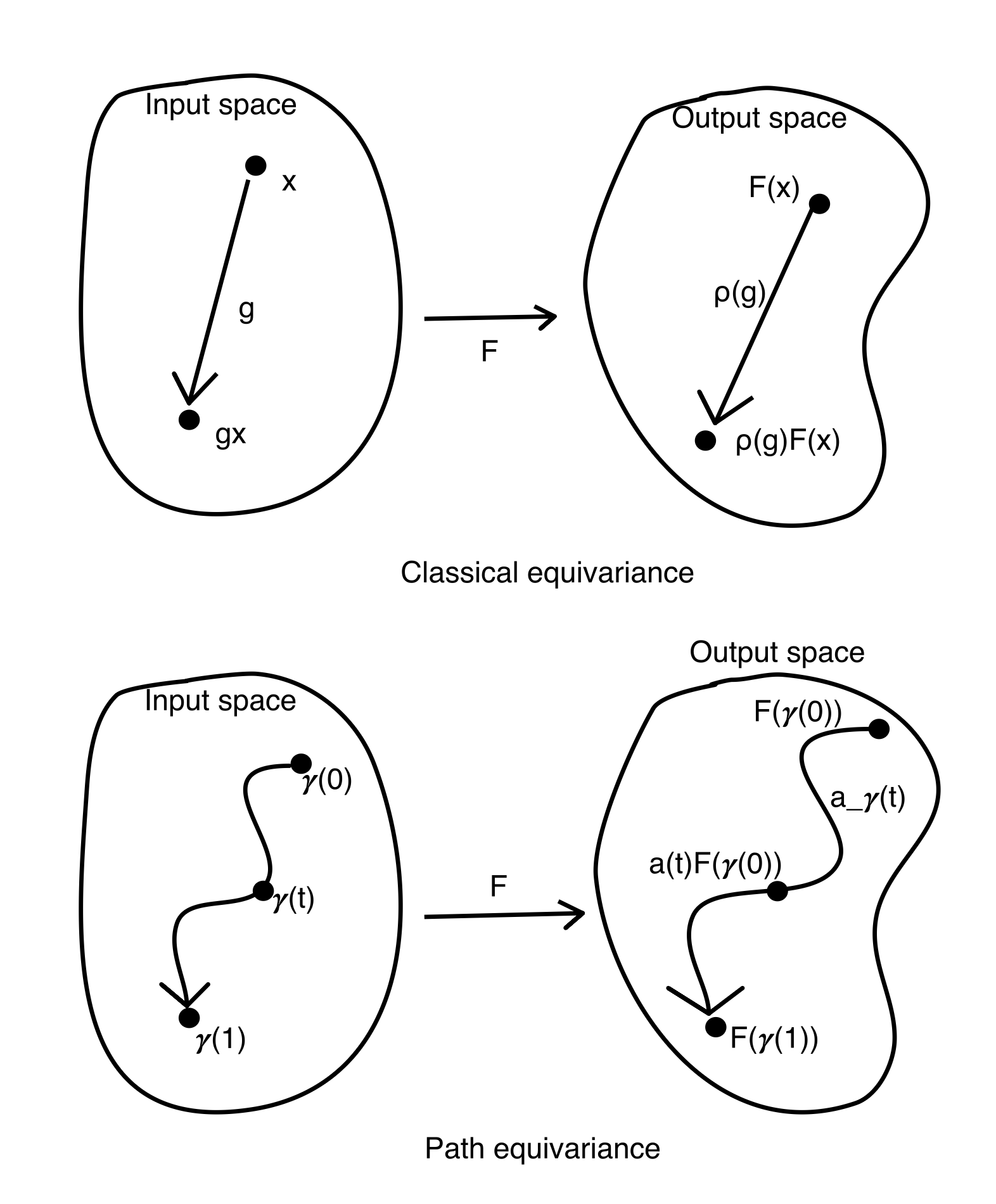
\[F(g \cdot x) = \rho(g) \cdot F(x) \quad \forall g \in G, \; x \in X\]This is powerful. It gives exact invariance guarantees and enables weight sharing. But it treats data points as isolated objects related by group actions. It says: “if I apply rotation $g$ to input $x$, the output should change by $\rho(g)$.” It says nothing about what happens between $x$ and $g \cdot x$, nothing about the continuous trajectory from one to the other.
Consider a face recognition system. Classical equivariance handles rotation well: a face rotated by 30° should produce a rotated feature map. But what about gradually morphing from one person’s face to another? That is a continuous path through data space, and we would like the network’s representation to change smoothly along it. Classical equivariance covers the rotation part perfectly, but morphing between faces is not a group action, and it has no mechanism for that.
Classical equivariance handles the group-structured variations beautifully, and that covers a lot of ground. But for the rest, for the continuous changes that don’t fit into any group, it has no mechanism to offer. Path equivariance picks up where it leaves off.
The idea: equivariance along paths
Path equivariance fills this gap. Instead of asking “how does the output change when I apply a group element to the input?”, it asks: as I trace a continuous path through input space, how does the output move through feature space?
Formally, a map $F: X \to Z$ is path equivariant if for every path $\gamma$ in a specified path system, there exists a continuous transport $a_\gamma: [0,1] \to A$ such that:
\[F(\gamma(t)) = a_\gamma(t) \cdot F(\gamma(0)) \quad \forall t \in [0,1]\]where $A$ is a group acting on the output space $Z$.
The intuition: as the input walks along a path $\gamma$, the output doesn’t jump around arbitrarily. It moves in a structured way, governed by the transport $a_\gamma(t)$. The transport tells us exactly how the representation evolves along the path.
The idea is intuitive and the formula is clean, but making it rigorous requires care: the path system must satisfy closure properties (reparametrization, concatenation), the transport must be continuous and compatible with composition, and the relationship between path equivariance and classical equivariance involves topological arguments about endpoint conditions and holonomy. The full technical development, including proofs, can be found in the thesis.
This is a strictly more general notion than classical equivariance. A classical G-equivariant map is automatically path equivariant for paths induced by the group action: if $\gamma(t) = g(t) \cdot x$ traces an orbit, then $a_\gamma(t) = \rho(g(t))$. But path equivariance can also handle paths that have nothing to do with any group: paths through content space, paths across different data manifolds, paths that no global symmetry relates.
Where does the manifold come from?
Before going further, let me clarify something that is easy to confuse. The path equivariance framework talks about “paths on manifolds.” But the manifold structure here does not come from the data manifold hypothesis. The manifolds in this framework come from the mathematical structure we impose.
The group $G$ is a manifold. If $G$ is a Lie group ($SO(2)$, $SO(3)$, $SE(3)$, etc.) it is by definition a smooth manifold. This is what makes pose paths well-defined: we can trace continuous curves through the group because the group itself is a smooth space. A path $\gamma_G(t)$ from the identity to some rotation $R$ is simply a curve on this group manifold.
The content space (which we will introduce later) $U = X/G$ is a manifold. When $G$ acts freely and properly on the data space $X$, the quotient $U = X/G$ inherits a manifold structure. This is what makes content paths well-defined: we can move continuously between equivalence classes (between “different objects at canonical pose”) because the quotient space is smooth.
So the paths in path equivariance are not vague appeals to “data living on a surface.” They are precisely defined curves on specific manifolds, the group manifold (Lie group) and the quotient manifold, whose existence follows from the algebraic and topological assumptions of the framework.
That said, the data manifold hypothesis provides important practical motivation. It tells us that paths through data space are meaningful objects worth studying, that nearby data points are related by smooth variation, not random jumps. And in implementation, the manifold hypothesis is what justifies using latent space interpolation, nearest-neighbor graphs, or generative model trajectories as proxies for “paths on the manifold.”
The infinitesimal perspective: what we gain and what we leave open
A reader with a Riemannian geometry background might notice something missing. The standard way to study manifolds is through tangent spaces and Jacobians, local linear approximations. The metric tensor, geodesics, curvature, parallel transport: all defined through the tangent bundle. This is the workhorse of differential geometry, and its power comes precisely from linearization. Once we’re in a tangent space, we can compute.
The path equivariance framework takes a different route. The PE condition $F(\gamma(t)) = a_\gamma(t) \cdot F(\gamma(0))$ is a statement about entire paths, not about tangent vectors at a point. The transport $a_\gamma(t)$ lives in a group $A$, not in a vector space. This is a deliberate choice, and it has both strengths and costs.
What the group-level formulation gains. Working with finite paths and group actions avoids assuming differentiability everywhere, avoids choosing coordinates, and directly captures global structure. The content-pose decomposition, the hierarchy from classical to homotopy to full path equivariance, the hard/soft constraint asymmetry: these are naturally topological results. They don’t need Jacobians and they don’t break when the manifold has singularities or non-smooth regions. The Lie group on the output side gives multiplicative, global structure that tangent spaces (which are merely additive, local) cannot provide.
What it costs. We lose the computational traction that linearization gives. In Riemannian geometry, we compute in tangent spaces: geodesics are ODE solutions, parallel transport is governed by connections (Lie-algebra-valued 1-forms), curvature measures the failure of infinitesimal transport to commute. By staying at the path level, path equivariance is more general but less directly computable.
The bridge that should exist. If we assume differentiability, the PE condition has a natural infinitesimal version. Differentiating $F(\gamma(t)) = a_\gamma(t) \cdot F(\gamma(0))$ at $t = 0$ gives:
\[dF(\dot{\gamma}(0)) = \dot{a}_\gamma(0) \cdot F(\gamma(0))\]The left side is the Jacobian of $F$ applied to the tangent vector $\dot{\gamma}(0)$, the standard Riemannian object. The right side is a Lie algebra element $\dot{a}_\gamma(0) \in \mathfrak{a}$ acting on $F(\gamma(0))$, which is nothing other than a connection on the output bundle, with the Lie algebra of $A$ as the structure algebra. The holonomy of this connection, the path-dependence of transport around closed loops, would correspond precisely to the curvature of the data manifold as seen through $F$.
This connects path equivariance to the classical differential geometry toolkit: paths and tangent vectors, groups and Lie algebras, holonomy and curvature are two levels of description of the same underlying structure. The path-level framework developed in this thesis provides the topological and global foundation; the infinitesimal version, which I have not fully developed, would provide the computational machinery. Connecting the two, showing precisely how the Jacobian of a path-equivariant map defines a connection and how the curvature of that connection governs the structure of learned representations, is a natural next step and one of the directions I am interested in pursuing.
Recovering classical equivariance as a special case
A natural question: when does path equivariance reduce back to classical group equivariance? The answer reveals the precise relationship between the two.
The key is the endpoint condition (my own terminology): if all paths leading to the same group element $g$ induce the same transport endpoint $a_\gamma(1)$, regardless of which path was taken, then the transport depends only on the endpoint, not on the path. In this case, the map $g \mapsto a_\gamma(1)$ becomes a well-defined group homomorphism $\rho: G \to A$, and we recover:
\[F(g \cdot x) = \rho(g) \cdot F(x)\]which is exactly classical equivariance.
This establishes a hierarchy of increasingly general equivariance notions:
- Classical G-equivariance: the endpoint condition holds universally. The path doesn’t matter, only the destination. This is what G-CNNs implement.
- Homotopy equivariance: paths that are homotopic (continuously deformable into each other) induce the same transport. The topological class of the path matters, but not its exact shape.
- Full path equivariance: different paths between the same endpoints can induce different transports. The geometry of the path itself matters.
Classical equivariance is the strongest (most constrained) case. Full path equivariance is the most general. The hierarchy tells us how much geometric structure our network respects, and correspondingly, how strong a prior we are encoding.
Content and pose: why the decomposition matters
The deepest application of path equivariance comes from decomposing the data manifold into two very different parts.
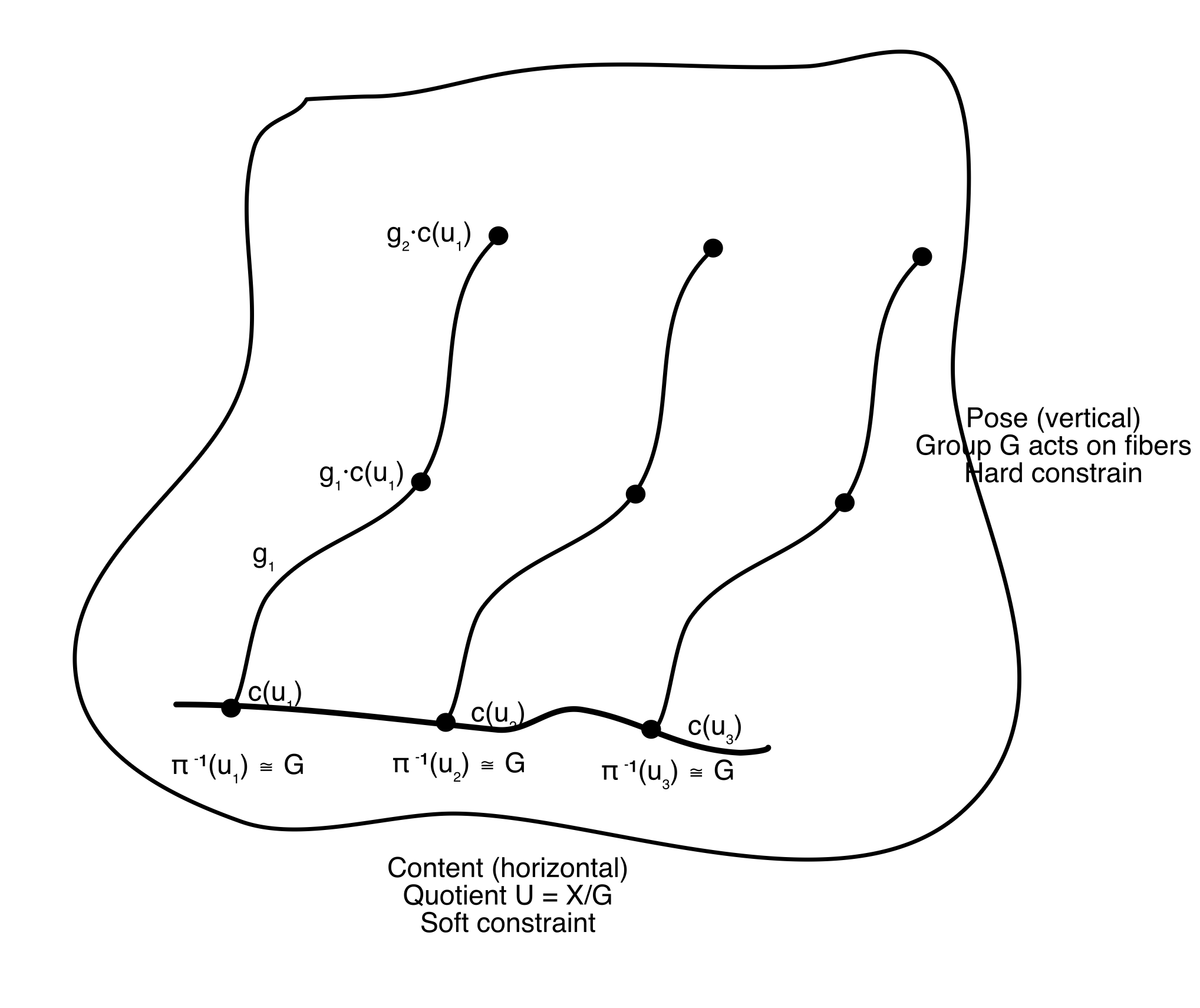
When a group $G$ acts freely on the data space $X$, the space factors into a principal $G$-bundle:
- Pose: the group orbit at each point, all the ways the data can be acted on by $G$ (e.g., all rotations of a given face)
- Content: the quotient $U = X/G$, what remains after factoring out the symmetry (e.g., the identity of the person, independent of pose)
Every data point decomposes uniquely as $x = g \cdot c(u)$: a content $u$ at a canonical pose, acted on by a group element $g$. This is not just abstract structure. It is the fiber bundle geometry of the data manifold, and it gives rise to two distinct kinds of paths.
Pose paths move within an orbit: $\gamma(t) = g(t) \cdot c(u)$, keeping content fixed and varying the group element. Rotating a face while keeping the person fixed. These paths carry group structure, and path equivariance on pose paths reduces (under the endpoint condition) to classical equivariance. Pose paths can be handled with hard constraints, exact weight sharing, the kind that CNNs implement.
Content paths move between orbits: $\gamma(t) = c(u(t))$, keeping the pose canonical and varying the content. Morphing from Alice’s face to Bob’s face at a fixed angle. These paths have no group structure; the content space $U$ is just a manifold, not a group. There is no homomorphism to exploit, no weight-sharing trick to deploy. Path equivariance on content paths can only be enforced as a soft constraint, a smoothness regularization encouraging the network’s output to vary continuously as content varies:
\[\mathcal{L}_{\text{smooth}} = \int \lVert\frac{d}{dt} F(c(\gamma_U(t)))\rVert^2 dt\]This asymmetry (hard constraints for pose, soft constraints for content) is not a design choice. It is a consequence of the mathematics. Pose lives in a group; content does not. The path equivariance framework makes this distinction precise and explains why certain invariances can be built into architectures (translation equivariance in CNNs) while others must be learned through training (similarity between different objects).
How would we actually implement this?
Groups are easy to represent in code: matrices, permutations, discrete sets. Manifolds and paths are harder. So how does path equivariance translate into something we can train?
Pose paths → architecture. The group-structured part uses existing equivariant networks directly. Steerable convolutions, group convolution layers, the entire G-CNN machinery applies. PENs contain classical equivariant networks as a component; nothing new is needed for pose.
Content paths → loss function. We don’t need an explicit manifold parameterization. We need pairs of nearby points and a loss that encourages smooth variation between them. The simplest approach is Laplacian regularization over a nearest-neighbor graph:
\[\mathcal{L}_{\text{smooth}} = \sum_{(i,j) \in \text{neighbors}} \lVert F(x_i) - F(x_j)\rVert^2.\]If a generative model is available, we can construct explicit interpolation paths in latent space and penalize non-smooth variation of $F$ along them. Methods like SimCLR and VICReg already enforce a version of this implicitly: augmentation invariance handles pose paths, while the contrastive or regularization objective structures content paths. The path equivariance framework gives a geometric interpretation of why these methods work.
The combined architecture for a Path Equivariant Network: an equivariant backbone (pose via hard constraints) plus a smoothness regularization in the loss (content via soft constraints).
What this framework contributes
Let me be explicit about what path equivariance adds beyond classical geometric deep learning.
It generalizes group equivariance without abandoning it. Classical G-NNs are a special case, not a competitor. The hierarchy (classical, homotopy, full path) lets us choose exactly how much geometric structure to encode, with classical equivariance as the strongest prior and full path equivariance as the weakest.
It connects fiber bundles to neural network design. The content-pose decomposition is not a metaphor. It is the principal bundle structure of the data manifold. The structure group $G$, the base space $U$, the local sections $c: U \to X$: these are the same objects that appear in gauge theory and differential geometry, now applied to characterize what a neural network should preserve.
It explains the hard/soft constraint asymmetry. This is perhaps the most practically relevant insight. Practitioners know that some invariances are easy to build in (convolution) and others must be learned (content similarity). The framework gives the mathematical reason: hard constraints correspond to group structure (pose), soft constraints correspond to manifold structure without group structure (content). If we want to know whether a given invariance can be hardcoded or must be regularized, check whether the relevant space of changes is a group.
Looking forward
The path equivariance framework opens several directions. The connection to holonomy (whether different paths between the same endpoints give different transports) links directly to the curvature of the data manifold. The homotopy equivariance level connects to the topology of the group, particularly the fundamental group $\pi_1(G)$. And the content-path smoothness constraint is, at its core, a Riemannian condition on the feature map, which connects to the manifold learning and information geometry literature.
The final article in this series takes one more step back: a category-theoretic perspective that unifies groups, manifolds, and path equivariance into a single framework where equivariance is naturality, and the entire apparatus becomes compositional.
Articles based on the thesis “Exploring the Structure in Deep Networks: Group, Manifold and Category Theory” (Aalto University, 2025).
Next: Part 4, a category theory perspective
Enjoy Reading This Article?
Here are some more articles you might like to read next: